Introduction

This is an analysis of the database dump provided by on 25/03/2021 by Simon Urbanek which is available to all at the previous link (If that fails it is also on this repository as R-bugs.sql .

The goal of this analysis is to identify good practices (or lack of them) to help people submitting better issues and implement helpful advice and rail guard on it to be helpful to the R core members.

Connecting to the database dump

First an initial exploration of the database and bug reports building on the previous analysis we convert some columns to dates:

library("lubridate")
## 
## Attaching package: 'lubridate'
## The following objects are masked from 'package:base':
## 
##     date, intersect, setdiff, union
date_columns_bugs <- c("creation_ts", "delta_ts", "lastdiffed", "deadline")
db_bugs <- tbl(db_bugzilla, "bugs") |> 
    collect() |> 
    mutate(across(!!date_columns_bugs, as.POSIXct, tz = "UTC", format = "%Y-%m-%d %H:%M:%OS"))
## Warning in .local(conn, statement, ...): Decimal MySQL column 24 imported as
## numeric
## Warning in .local(conn, statement, ...): Decimal MySQL column 25 imported as
## numeric
## Warning in .local(conn, statement, ...): Decimal MySQL column 24 imported as
## numeric
## Warning in .local(conn, statement, ...): Decimal MySQL column 25 imported as
## numeric
db_bugs |> 
    ggplot() +
    geom_point(aes(creation_ts, bug_id, color = bug_id)) +
    labs(title = "Bugs created", y = "ID", x = "Creation") +
    guides(color = "none")
## Warning: Removed 14 rows containing missing values (geom_point).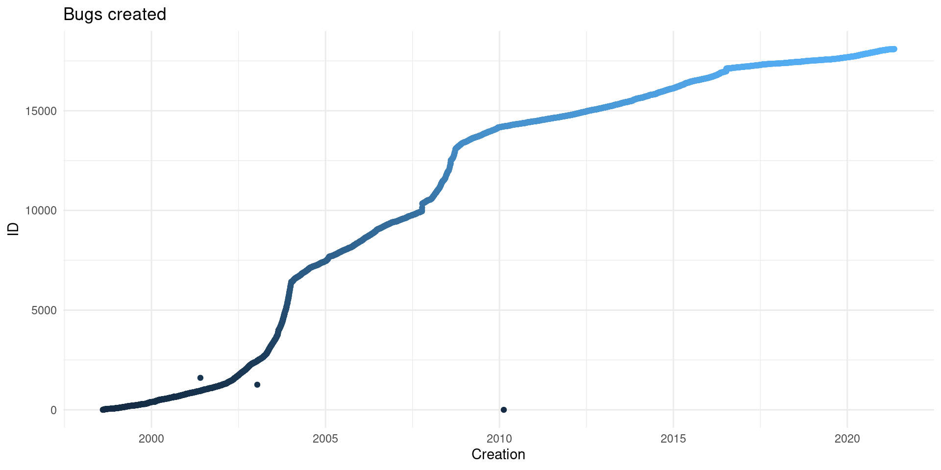

There are also three points that do not follow the general expectations¹.

Exploring outliers

These three odd bug reports that are not consistent with the path position and numbering of the other bug reports need some exploration.

special_bugs <- c(1, 1261, 1605)

Not clear what happens on 1261 or 1605, as there isn’t anything that provides a clue on what could have happened.

However, if we look at the first bug report on the website you’ll realize the first bug is testing Bugzilla! That first bug was made on 2010, in addition some bugs with later id have earlier creation date and even some without any submission date.

Perhaps these bugs were reported by some account with different characteristics. If we check who has been reporting the bugs we see this top users reporting bugs:

db_bugs |> 
  count(reporter, sort = TRUE) |> 
  head() |> 
  knitr::kable(align = "c", col.names = c("User", "Bugs reported"))

User	Bugs reported
2	3594
1036	73
963	70
1044	62
1056	60
3256	52

If we go to any of the bugs reported by user 2 we’ll find out that the bug report is reported by “Jitterbug compatibility account” and that many comment on the issues are from the same account. That account reported many bugs from before the first bug was added on Bugzilla. In conclusion we can estimate that approximately from 1998-08-07 bugs are filled on Bugzilla and previously were reported on Jitterbug.

Jitterbug and Bugzilla

Looking at the mailing list there are some report of some troubles migrating the bugs and it is not completely clear from the database when the switch happened. But it is clear that the R project moved from Jitterbug to Bugzilla, so the reporting of bugs changed too. If we explore the bug status and the bug resolution depending on if it was reported by user 2 or not we see the following visualization.

db_bugs2 <- db_bugs |> 
  mutate(reported_on = ifelse(reporter == 2, "Jitterbug", "Bugzilla"),
         reported_on = factor(reported_on, levels = c("Jitterbug", "Bugzilla")))
moving_date <- max(db_bugs2$creation_ts[db_bugs2$reported_on == "Jitterbug"], 
                   na.rm = TRUE)
db_bugs2 <- db_bugs2 |> 
  mutate(modified_on = ifelse(delta_ts >= moving_date, "Bugzilla", "Jitterbug")) |> 
  mutate(modified_on = ifelse(is.na(modified_on), "Jitterbug", modified_on)) |> 
  mutate(modified_on  = ifelse(reported_on == "Bugzilla", "Bugzilla", modified_on))

db_bugs2 |> 
  count(bug_status, resolution, reported_on, sort = TRUE) |> 
  mutate(resolution = ifelse(resolution == "", "Not resolved", resolution)) |> 
  ggplot() +
  geom_tile(aes(bug_status, resolution, fill = n)) +
  facet_wrap(~reported_on) +
  labs(fill = "Bugs", x = "Status", y = "Resolution")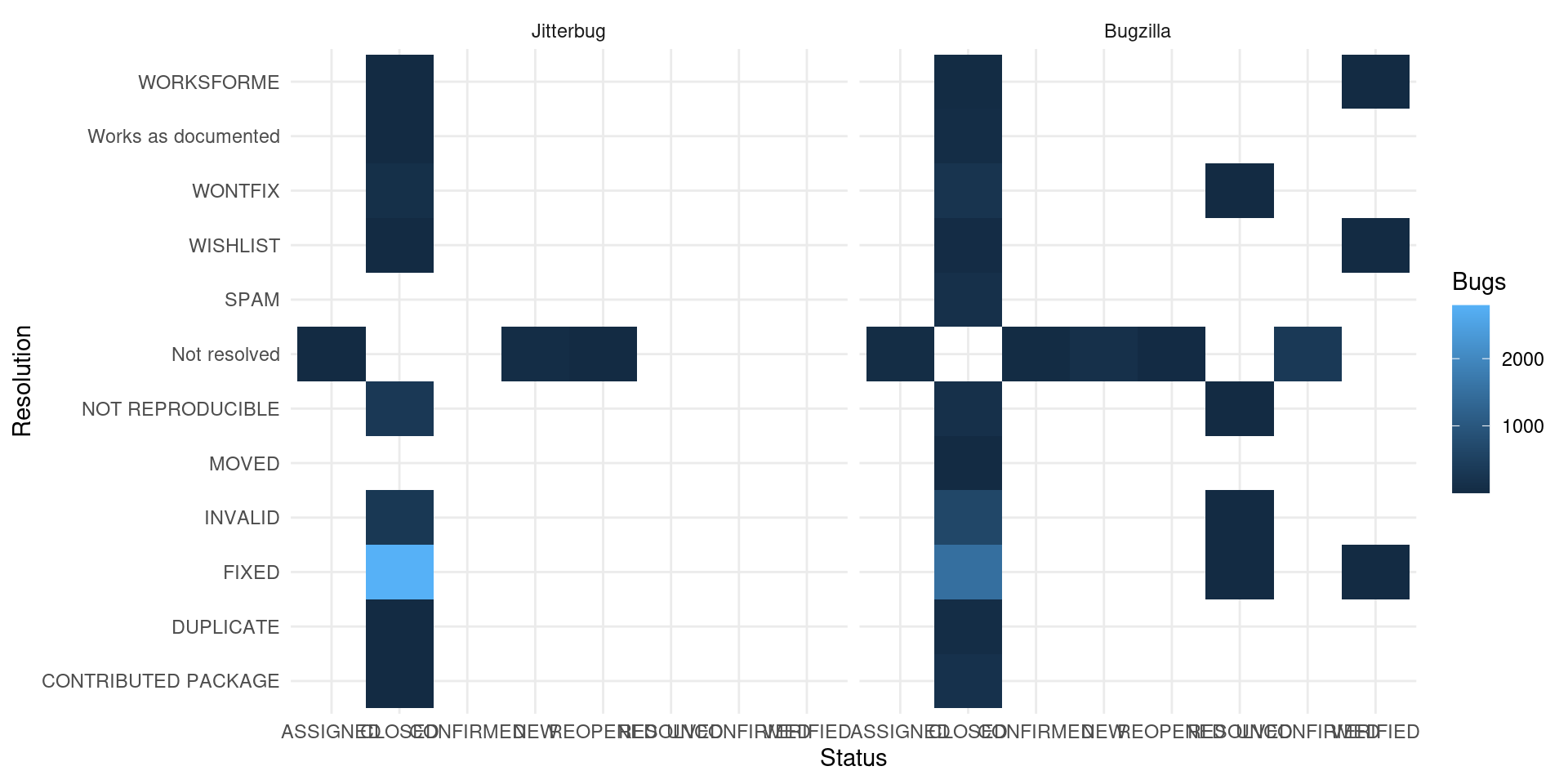

If we focus on the bugs that are not spam and where was the last update we see a complete different picture of status and resolutions:

db_bugs3 <- db_bugs2 |> 
  filter(resolution != "SPAM") |> 
  mutate(bug_severity = fct_relevel(bug_severity, 
                                    c("trivial", "minor", "normal", "major", "blocker", "enhancement")))
db_bugs3 |> 
  count(bug_severity, bug_status, modified_on, sort = TRUE) |> 
  ggplot() +
  geom_tile(aes(bug_severity, bug_status, fill = n)) +
  facet_wrap(~modified_on) +
  labs(x = "Severity", y = "Status", fill = "Bugs")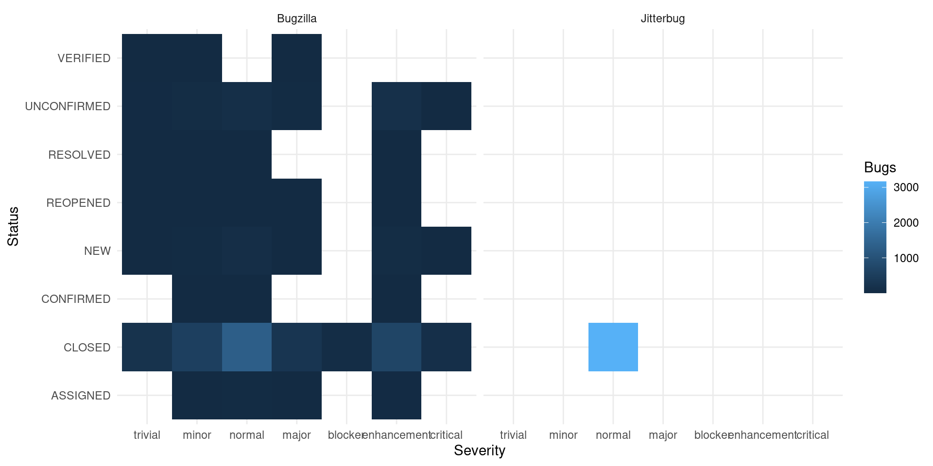

The information about the resolution and status of bugs on Jitterbug is missing from the database. (There is some reports of changes on the comments though)

db_bugs4 <- db_bugs3 |> 
  filter(reported_on == "Bugzilla",
         bug_id != 1)
db_bugs4 |> 
  count(bug_severity, bug_status, sort = TRUE) |> 
  ggplot() +
  geom_tile(aes(bug_severity, bug_status, fill = n)) +
  labs(x = "Severity", y = "Status", fill = "Bugs", title = "Bugs on Bugzilla")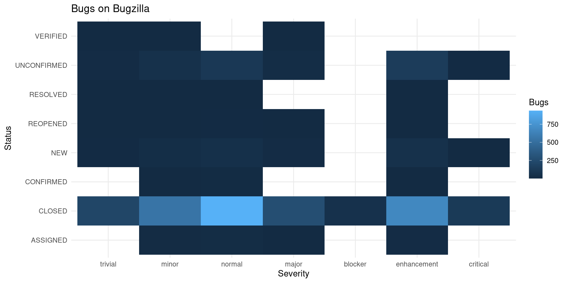

If we focus only on Bugzilla, most bugs are “normal” but some classification is done on the status and severity. Should someone help classify the bugs to different severity to prioritize working on them?

First time

Looking at when for the first time some field was used might provide some insight on changes on the way that the bug report system has been modified.

first_time <- function(b, cat) {
  b |> 
    filter(bug_id != 1) |> 
    group_by({{cat}}) |> 
    summarise(bug_id = bug_id[which.min(creation_ts)],
              creation_ts = min(creation_ts, na.rm = TRUE), n = n(), .groups =  "drop") |> 
    arrange(creation_ts, bug_id) |> 
    mutate(creation_ts = lubridate::date(creation_ts)) |> 
    mutate(bug_id = paste0("[", bug_id,
                           "](https://bugs.r-project.org/show_bug.cgi?id=", bug_id, ")"))
}

first_time(db_bugs3, bug_status) |> 
  knitr::kable(align = "c", col.names = c("Bug", "Status", "First report", "Total bugs"))

Bug	Status	First report	Total bugs
CLOSED	3	1998-08-07	6334
NEW	408	2000-01-28	172
ASSIGNED	1161	2001-11-07	43
REOPENED	8192	2005-10-09	12
UNCONFIRMED	14335	2010-07-14	324
VERIFIED	14452	2010-12-04	3
RESOLVED	16576	2015-10-22	9
CONFIRMED	16648	2015-12-29	13

Surprisingly the CONFIRMED and RESOLVED status wasn’t used until 2015. I’ve heard that this was added relatively lately by one R core member.

first_time(db_bugs3, resolution) |> 
  knitr::kable(align = "c",
               col.names = c("Resolution", "Bug", "First report", "Total bugs"))

Resolution	Bug	First report	Total bugs
FIXED	3	1998-08-07	4304
WONTFIX	105	1999-01-29	336
	408	2000-01-28	564
INVALID	424	2000-02-08	935
Works as documented	837	2001-02-01	50
NOT REPRODUCIBLE	848	2001-02-13	434
WISHLIST	961	2001-05-31	36
CONTRIBUTED PACKAGE	1729	2002-07-02	157
WORKSFORME	2888	2003-04-30	24
DUPLICATE	8725	2006-03-29	68
MOVED	16182	2015-02-02	2

All resolutions were fairly soon used except the moved one.

first_time(db_bugs3, version) |> 
  knitr::kable(align = "c", col.names = c("Version", "Bug", "First report", "Total bugs"))

Version	Bug	First report	Total bugs
old	3	1998-08-07	3637
R 3.1.1	1662	2002-06-13	75
R 3.0.2	2048	2002-09-20	152
R 2.14.0	6899	2004-05-21	47
R 3.0.1	7991	2005-07-06	116
R 2.15.1	13684	2009-05-01	58
R 2.y.z	14229	2010-03-13	213
R 2.10.x	14231	2010-03-16	50
R 2.12.0	14272	2010-04-27	48
R 2.x	14277	2010-04-30	13
R 2.11.1	14322	2010-06-24	59
R-devel (trunk)	14359	2010-08-13	615
R 2.12.1	14464	2010-12-20	28
R 2.12.2	14522	2011-03-07	19
R 2.13.0	14559	2011-04-19	40
R 2.13.1	14605	2011-06-14	41
R 2.13.2	14656	2011-08-11	17
R 3.0.0	14682	2011-09-20	102
R 2.15.0	14832	2012-03-04	52
R 2.15.x	14875	2012-04-10	204
R 2.14.2	14879	2012-04-13	10
R 3.6.xx	14905	2012-05-03	87
R 3.1.0	15072	2012-10-12	104
R 3.1.2	15522	2013-10-31	142
R 3.0.3	15725	2014-03-26	10
R 3.4.0	16086	2014-11-24	36
R 3.2.0	16321	2015-04-17	73
R 3.1.3	16322	2015-04-17	19
R 3.2.1	16327	2015-04-22	76
R 3.2.2	16558	2015-10-08	65
R 3.2.3	16651	2016-01-03	69
R 3.2.4	16760	2016-03-12	23
R 3.2.4 revised	16775	2016-03-20	15
R 3.3.*	16776	2016-03-21	164
R 3.5.2	16877	2016-05-04	10
R 3.4.1	17325	2017-08-09	30
R 3.4.3	17384	2018-02-01	15
R 3.5.0	17405	2018-04-12	145
R 3.4.4	17408	2018-04-18	7
R 3.5.1	17468	2018-09-12	17
R 3.5.3	17582	2019-07-18	2
R 4.0.0	17773	2020-04-28	26
R 4.0.x	17775	2020-04-28	179

Some bugs reports of previous versions (not sure if version-specific) happen later than on new versions. Probably is people using previous version that report problems they found.

first_time(db_bugs3, bug_severity) |> 
  knitr::kable(align = "c", col.names = c("Severity", "Bug", "First report", "Total bugs"))

Severity	Bug	First report	Total bugs
normal	3	1998-08-07	4700
enhancement	616	2000-07-25	876
critical	2048	2002-09-20	122
major	9807	2007-07-25	306
minor	14229	2010-03-13	626
trivial	14252	2010-04-10	228
blocker	14265	2010-04-22	52

On 2010 it seems that minor and trivial issues were started to be reported.

component_names <- c("2" = "Accuracy", 
                     "3" = "Analyses",
                     "4" = "Graphics",
                     "5" = "Installation",
                     "6" = "Low-level", 
                     "8" = "S4methods", 
                     "7" = "Misc",
                     "9" = "System-specific",
                     "10" = "Translations",
                     "11" = "Documentation", 
                     "12" = "Language",
                     "13" = "Startup", 
                     "14" = "Models",
                     "15" = "Add-ons", 
                     "16" = "I/O",
                     "17" = "Wishlist", 
                     "18" = "Mac GUI / Mac specific", 
                     "19" = "Windows GUI / Window specific" 
                     )
first_time(db_bugs3, component_id) |> 
  mutate(component_id = component_names[as.character(component_id)]) |> 
  knitr::kable(align = "c", col.names = c("Component", "Bug", "First report", "Total bugs"))

Component	Bug	First report	Total bugs
Language	3	1998-08-07	411
Models	4	1998-08-10	256
System-specific	7	1998-08-17	284
I/O	12	1998-08-19	301
Documentation	19	1998-08-19	712
Startup	21	1998-08-21	46
Analyses	26	1998-08-31	325
Low-level	37	1998-09-06	662
Graphics	38	1998-09-06	542
Windows GUI / Window specific	46	1998-09-24	438
Installation	58	1998-10-30	335
Misc	91	1999-01-09	1146
Wishlist	105	1999-01-29	462
Add-ons	122	1999-02-18	347
Accuracy	138	1999-03-10	327
Mac GUI / Mac specific	1015	2001-07-06	236
S4methods	4073	2003-09-05	55
Translations	7841	2005-05-06	25

There seems to be interest on translations since 2005, quite early on the development of R.

first_time(db_bugs3, rep_platform) |> 
  knitr::kable(align = "c", col.names = c("Platform", "Bug", "First report", "Total bugs"))

Platform	Bug	First report	Total bugs
All	3	1998-08-07	3752
ix86 (32-bit)	47	1998-09-24	1297
x86_64/x64/amd64 (64-bit)	1662	2002-06-13	1025
Other	14272	2010-04-27	813
PowerPC	14548	2011-04-05	20
SGI	14849	2012-03-18	1
Sparc	16514	2015-08-18	2

I don’t know what these platforms mean, but there seems that every 3 years there’s a new platform report.

first_time(db_bugs3, op_sys) |> 
  knitr::kable(align = "c", col.names = c("OS", "Bug", "First report", "Total bugs"))

OS	Bug	First report	Total bugs
All	3	1998-08-07	2150
Solaris	4	1998-08-10	204
Other	7	1998-08-17	640
Linux-Fedora	12	1998-08-19	124
Linux-Debian	15	1998-08-20	114
Linux	43	1998-09-19	1287
Windows 32-bit	47	1998-09-24	1190
Mac OS X v10.5	697	2000-10-16	85
FreeBSD	1613	2002-05-30	22
Linux-Ubuntu	2048	2002-09-20	168
Windows 64-bit	6762	2004-04-13	512
Mac OS X v10.4	7973	2005-06-28	66
AIX	13440	2009-01-09	14
Mac OS X v10.8	13684	2009-05-01	48
Mac OS X v10.6	14226	2010-03-02	87
unix-other	14463	2010-12-18	9
Mac OS X v10.7	14670	2011-09-08	25
Linux-RHEL	15037	2012-08-30	21
OS X Mavericks	15520	2013-10-30	75
OS X Yosemite	16375	2015-05-08	27
OS X El Capitan	16911	2016-05-17	28
macOS	17782	2020-05-04	14

Multiple issues on each component, many are reported on Windows and some are reported for all OS.

Spam

As seen there are some bugs classified as APM. This was a new resolution on Bugzilla. In order to explore this we can check out the missing issues (bug ids that are not present but that later ids are) and spam to see what happened:

missing_ids <- (db_bugs2$bug_id - lag(db_bugs2$bug_id) -1)
missing_ids[db_bugs2$resolution == "SPAM"] <- 1
missing_ids[is.na(missing_ids)] <- 0
data.frame(bug = db_bugs2$creation_ts, 
           spam = missing_ids, 
           reported_on = db_bugs2$reported_on) |>
  filter(spam != 0) |> 
  ggplot() +
  geom_point(aes(bug, spam, color = reported_on, shape = reported_on)) +
  # Date from https://www.r-project.org/bugs.html +1 day of effect
  geom_vline(xintercept = as_datetime("2016-07-10")) + 
  labs(title = "Battle against spam",
       y = "Missing bugs or SPAM",
       col = "Site",
       shape = "Site",
       x = element_blank())
## Warning: Removed 5 rows containing missing values (geom_point).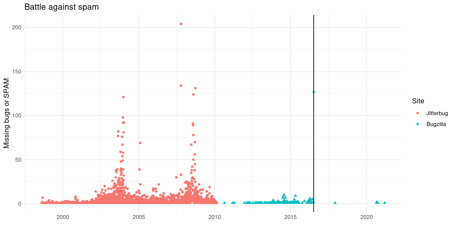

There are two waves of missing or spam bugs on Jitterbug and later less problems on the move to Bugzilla.

It could also be that there were some problem migrating bugs from Jitterbug and some issues were not correctly moved, or simply that some issues are omitted due to the security vulnerability policy to omit them from appearing on the database. Since the move to Bugzilla there was some constant but low volume spam issue compared to Jitterbug.

But I think that the wave of spam or missing on Bugzilla that is the same day a new SPAM policy was enacted (vertical line) shows that these numbers show mostly spam. After the new policy to ask permission for an account, started where the vertical line is, has worked very well. There seem to be less missing/spam bugs lately. Given all that we will omit the spam bugs from now on. They are not really bug reports nor report or have something of quality to learn from them.

Attachments

If we look at the attachments we might get some information about the kind of patches, packages, or reproducible examples that are provided.

db_attachments <- tbl(db_bugzilla, "attachments") |> 
  collect() |> 
  mutate(across(c("creation_ts", "modification_time"), as.POSIXct, format = "%Y-%m-%d %H:%M:%OS", tz = "UTC"))
db_attachments_bugs <- db_bugs3 |> 
    left_join(db_attachments, by = "bug_id", suffix = c(".bug", ".at"))
db_attachments_bugs |> 
  group_by(bug_id, reported_on) |> 
  summarize(attachments = sum(!is.na(creation_ts.at))) |> 
  ungroup() |> 
  ggplot() +
  geom_bar(aes(attachments, fill = reported_on)) +
  facet_wrap(~reported_on, scales = "free_x") +
  labs(fill = "Reported on")
## `summarise()` has grouped output by 'bug_id'. You can override using the `.groups` argument.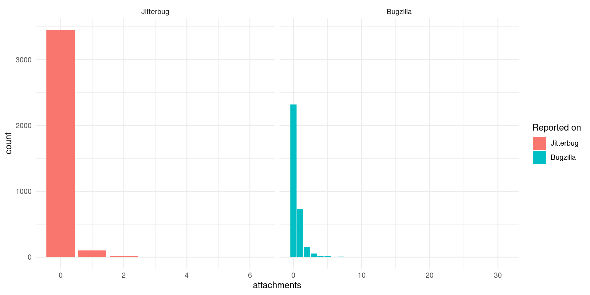

Most bug reports don’t have attachments! So this means that they are just some reporting of a problem which the R core then needs to understand and figure a solution. Surprisingly some bug reports have many attachments, this might be related to a refinement on patches or exploring several options.

db_attachments_bugs |> 
  group_by(bug_id) |> 
  summarize(have_attachments = any(!is.na(creation_ts.at)),
            x = creation_ts.bug,
            y = bug_id,
            reported_on = reported_on) |> 
  ungroup() |> 
  count(reported_on, have_attachments, sort = TRUE) |>
  knitr::kable(align = "c",
               col.names = c("Reported on", "Attachments", "Bugs"))
## `summarise()` has grouped output by 'bug_id'. You can override using the `.groups` argument.

Reported on	Attachments	Bugs
Jitterbug	FALSE	3453
Bugzilla	FALSE	2321
Bugzilla	TRUE	1592
Jitterbug	TRUE	201

Proportionally there are more attachments on Bugzilla.

Perhaps some attachments weren’t moved from Jitterbug, but it seems that the large difference might be from an increase in participation and patches proposed on Bugzilla.

attachments_type <- db_attachments_bugs |> 
  group_by(bug_severity, bug_status, bug_id, reported_on) |> 
  summarize(have_attachments = any(!is.na(creation_ts.at)),
            n_attachments = sum(!is.na(creation_ts.at))/n()) |> 
  ungroup() |> 
  group_by(bug_severity, bug_status, reported_on) |> 
  count(n_attachments) |> 
  mutate(attached = n_attachments > 0) |>
  group_by(bug_severity, bug_status, reported_on) |> 
  mutate(p = n/sum(n)) |> 
  filter(attached)
## `summarise()` has grouped output by 'bug_severity', 'bug_status', 'bug_id'. You can override using the `.groups` argument.

attachments_type |> 
  filter(reported_on == "Bugzilla") |> 
  ggplot() +
  geom_tile(aes(bug_severity, bug_status, fill = p)) +
  scale_fill_viridis_c(labels = scales::percent_format(), limits = c(0, 1)) +
  labs(title = "Percentage of issues with attachments",
       subtitle = "On Bugzilla", fill = "Attachments",
       x = "Severity", y = "Status")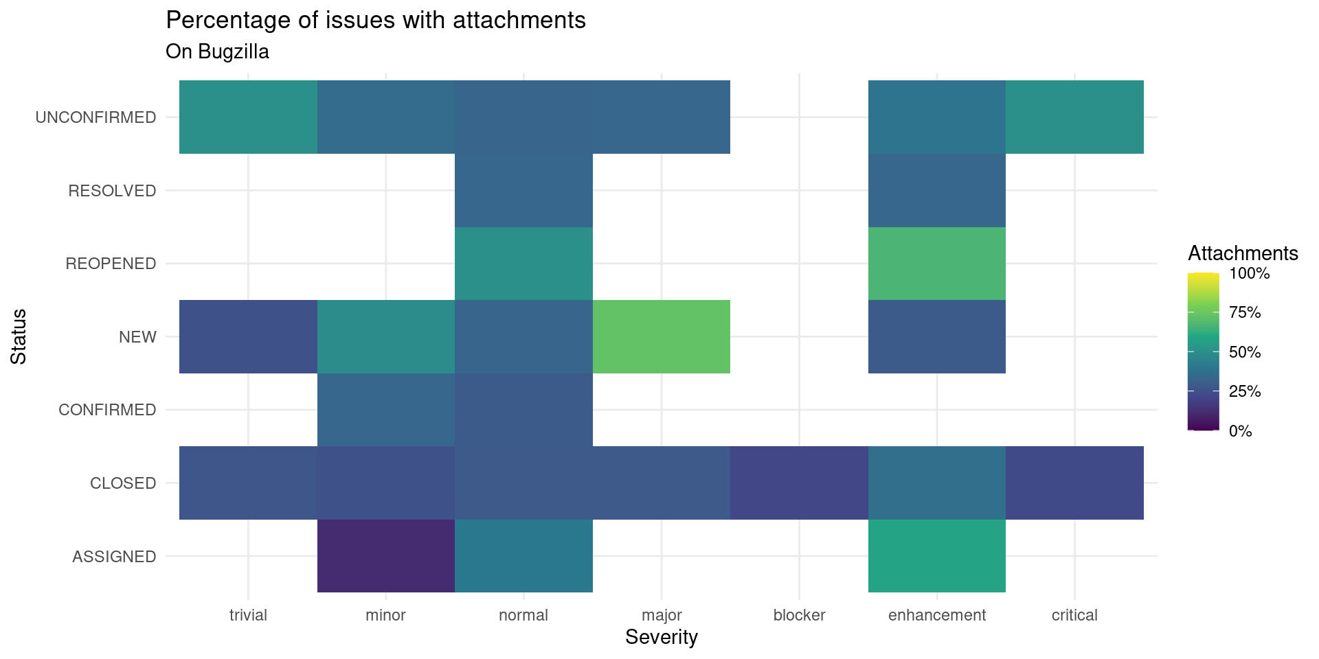

Looking at which severity has more attachments and which status, is kind of confusing. Probably the attachment is more related to who is reporting the bug or people proposing solutions.

What is the time between posting the bug and the attachments?

attachment_time <- db_attachments_bugs |> 
    filter(!is.na(creation_ts.at),
           !is.na(creation_ts.bug)) |> 
    filter(reported_on == "Bugzilla") |> 
    mutate(t = creation_ts.at - creation_ts.bug,
           mt0 = t == 0)
attachment_in <- attachment_time |>
  filter(!mt0) |> 
  group_by(bug_id) |> 
  arrange(t) |> 
  slice_head(n = 1) |> 
  ungroup() |> 
  summarize(attachment_in = as.numeric(median(t), units = "hours")) |> 
  pull(attachment_in)
attachment_time |> 
  count(mt0) |> 
  mutate(p = round(n/sum(n)*100, 2)) |> 
  knitr::kable(col.names = c("Attachment on  opening", "Bugs", "%"), align = "c")

Attachment on opening	Bugs	%
FALSE	881	55.34
TRUE	711	44.66

Bugs with attachments on opening are almost 50% and when not on opening there is an attachment in around 19.63 hours.

Exploring some issues like 7022 it seems that changes on tagging and notes is posted as comments. If we want to look at comments and time between changes this will distort the results, even more, we want to improve bug reports for Bugzilla not jitterbug. So from now we will only work with Bugzilla bugs.

db_attachments_bugs |> 
  filter(reported_on == "Bugzilla",
         !is.na(mimetype)) |> 
  group_by(ispatch) |> 
  count(mimetype, sort = TRUE) |> 
  head() |> 
  knitr::kable(row.names = FALSE, align = "c",
               col.names = c("Is patch?", "mimetype", "Bugs"), digits = 0)

Is patch?	mimetype	Bugs
1	text/plain	773
0	text/plain	287
0	application/octet-stream	128
0	image/png	89
0	application/pdf	42
0	application/x-gzip	42

Most files attached are not patches, even not all plain text files attached are patches. They might be packages showing the issues, plots where the deffect is apparent or files with data for examples.

db_attachments_bugs |> 
  filter(reported_on == "Bugzilla",
         !is.na(mimetype)) |> 
  group_by(ispatch) |> 
  count(submitter_id, sort = TRUE) |> 
  ggplot() +
  geom_bar(aes(n, fill = factor(ispatch, labels = c("Patch", "Other"),
                                levels = c(1, 0)))) +
  labs(fill = "", y = "Users", x = "Attachments")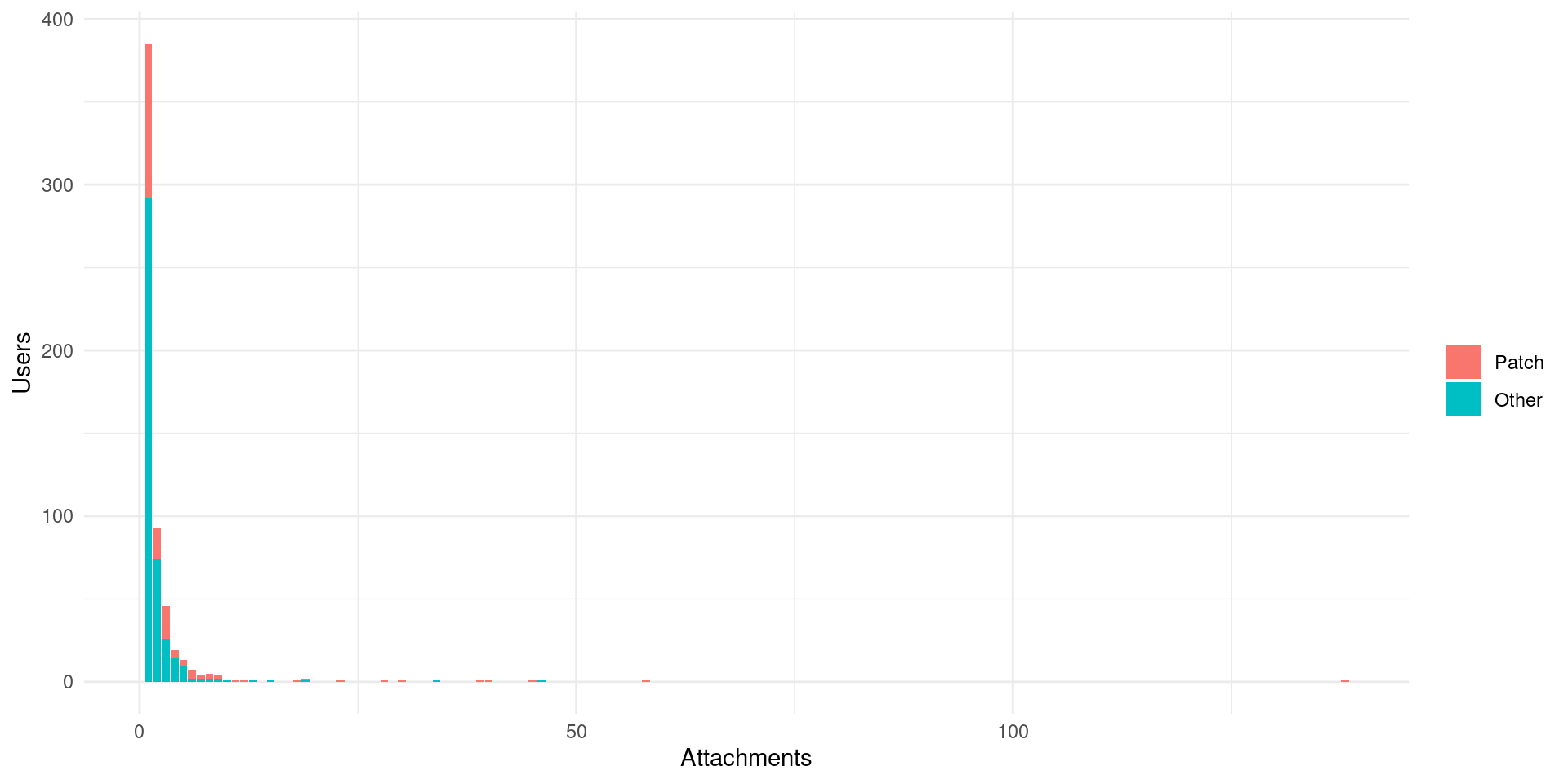

Most people submit just one file and few submit more than file. Of those there are very few patches (as detected by the system) This might suggest that people either don’t find bugs easy to patch, (or know how to do that) or they provide patches through other ways (r-devel mailing list for instance).

Activity on bugs reports

The bugs reports receive some attention and change if people performs some action through the Bugzilla tracker. If we look at the changes and addition to bugs we might get some idea of what is needed or missing from bug reports:

db_activity <- tbl(db_bugzilla, "bugs_activity") |> 
  collect() |> 
  mutate(bug_when = as.POSIXct(bug_when, tz = "UTC", format = "%Y-%m-%d %H:%M:%OS")) |> 
  filter(bug_id %in% db_bugs4$bug_id)


field_names <- c(
  "2" = "Summary", 
  "5" = "Version", 
  "6" = "Hardware", 
  "7" = "URL",
  "8" = "OS", 
  "9" = "Status", 
  "11" = "Keywords", 
  "12" = "Resolution",
  "13" = "Severity", 
  "14" = "Priority", 
  "15" = "Component", 
  "16" = "Assignee",
  "20" = "CC", 
  "21" = "Depends on", 
  "22" = "Blocks", 
  "23" = "Attachment description",
  "25" = "Attachment mime type", 
  "26" = "Attachment is patch",
  "27" = "Attachment is obsolete", 
  "34" = "?", 
  "36" = "Ever confirmed",
  "39" = "Group", 
  "40" = "?", 
  "41" = "?", 
  "42" = "Deadline", 
  "47" = "?",
  "54" = "See Also"
)

db_activity2 <- db_activity |> 
  mutate(field = field_names[as.character(fieldid)])

db_activity2 |> 
  count(field, adding = ifelse(removed %in% c("", "0"), "Added", "Changed")) |>
  tidyr::pivot_longer(cols = adding,
                      names_to = "type", values_to = "value") |> 
  ggplot() +
  geom_tile(aes(value, fct_reorder(field, n, .fun = sum), fill = n)) +
  scale_fill_viridis_c(trans = "log10") +
  labs(x = element_blank(), y = element_blank(), title = "Actions on bugs",
       fill = "Bugs")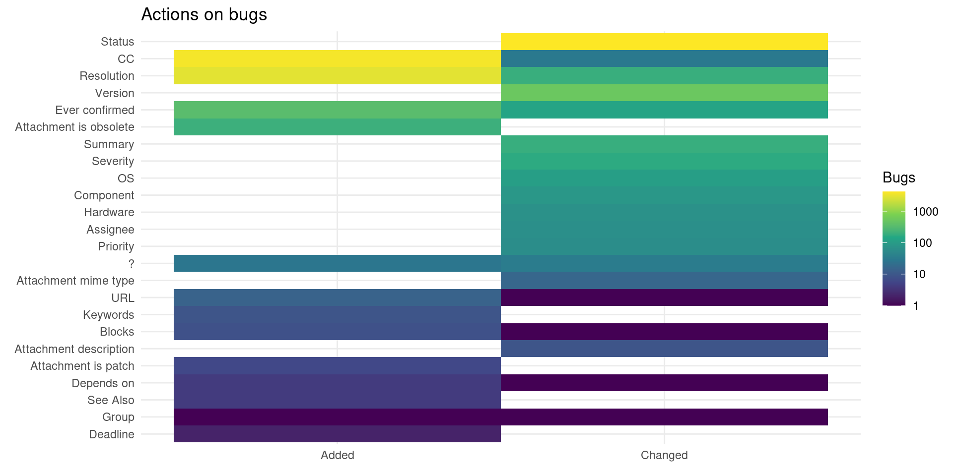

Changes on bug are on status, or people subscribing (usually via commenting on the issue). The ones that users can work to improve and provide better version description and title (Summary), followed by the severity, assigning to the right group, choosing the right OS, component and hardware.

db_activity2 |> 
  count(bug_id, sort = TRUE) |> 
  count(n) |> 
  mutate(n = as.factor(n)) |> 
  ggplot() +
  geom_col(aes(x = n, y = nn)) +
  labs(x = "Activity", y = "Bugs", title = "Activity on bugs")
## Storing counts in `nn`, as `n` already present in input
## ℹ Use `name = "new_name"` to pick a new name.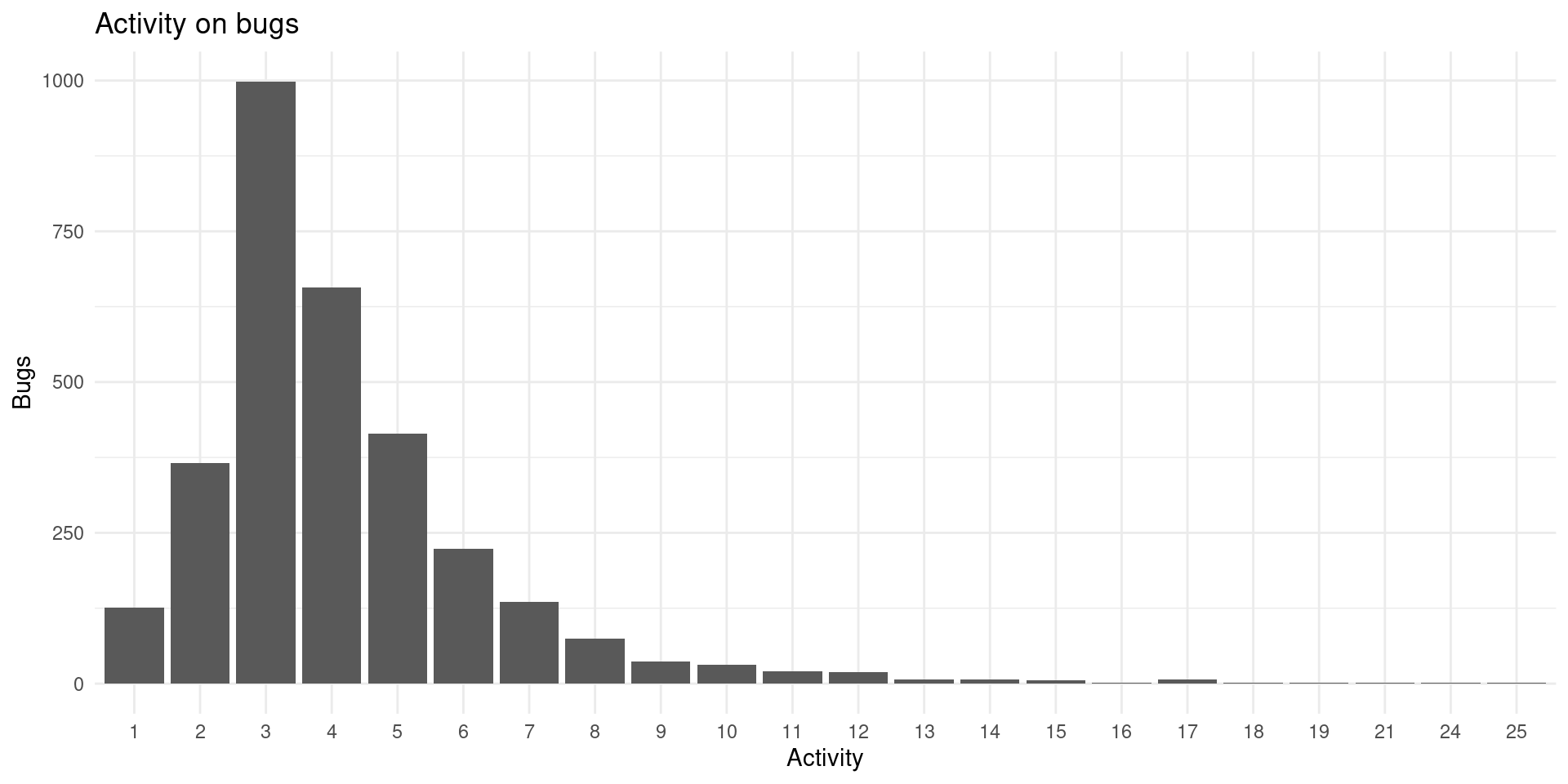

Usually issues receive around 4 modifications, probably status, CC and resolution and version. Let’s check which are the fields most often changed:

db_activity2 |> 
    select(bug_id, field) |> 
    arrange(bug_id, field) |> 
    group_by(bug_id) |> 
    summarize(fields = list(unique(field))) |> 
    ungroup() |> 
    count(fields, sort = TRUE) |> 
    mutate(size = lengths(fields)) |> 
    filter(n > 100) |> 
    pull(fields) |> 
    vapply( paste, collapse = ", ", FUN.VALUE = character(1L))
## [1] "CC, Resolution, Status"                
## [2] "Resolution, Status"                    
## [3] "CC, Resolution, Status, Version"       
## [4] "CC, Ever confirmed, Resolution, Status"
## [5] "CC"                                    
## [6] "Resolution, Status, Version"

Adding someone as CC usually means that they have commented. So surprisingly some change resolution but no one else comments. While 3 of the 5 more common activities involve adding someone as CC.

The components also change quite frequently:

db_activity2 |> 
  filter(field == "Component") |> 
  group_by(added) |> 
  count(sort = TRUE) |> 
  head() |> 
  knitr::kable(col.names = c("Component", "Bugs"))

Component	Bugs
Wishlist	15
Accuracy	8
Low-level	8
Misc	8
Mac GUI / Mac specific	6
Windows GUI / Window specific	6

Generally it seems that components are changed to make them wishlist.

db_activity2 |> 
  filter(field == "OS") |> 
  group_by(added) |> 
  count(sort = TRUE) |> 
  head() |> 
  knitr::kable(col.names = c("OS", "Bugs"))

OS	Bugs
All	60
Windows 64-bit	15
Linux	5
Mac OS X v10.9	4
Windows 32-bit	4
Linux-Ubuntu	3

And OS changes are to make it either more specific or more frequently more general.

db_activity2 |> 
  filter(field == "Hardware") |> 
  group_by(added) |> 
  count(sort = TRUE) |> 
  head() |> 
  knitr::kable(col.names = c("Hardware", "Bugs"))

Hardware	Bugs
All	48
x86_64/x64/amd64 (64-bit)	18
ix86 (32-bit)	1
PowerPC	1

Hardware changes seems to be the report more general.

However, as seen the numbers of these changes are quite low. The highest are the status, resolution and adding someone to the list of CC. This usually happens when someone comments. So how many comments are on issues?

Comments on bug reports

Looking at the comments on bug reports we we’ll see how much exchange is there usually:

db_comments <- db_bugzilla |> 
  tbl("longdescs") |> 
  collect() |> 
  mutate(bug_when = as.POSIXct(bug_when, tz = "UTC", 
                               format = "%Y-%m-%d %H:%M:%OS")) |> 
  filter(bug_id %in% db_bugs4$bug_id)
## Warning in .local(conn, statement, ...): Decimal MySQL column 4 imported as
## numeric

## Warning in .local(conn, statement, ...): Decimal MySQL column 4 imported as
## numeric

db_comments |> 
  count(bug_id) |> 
  count(n) |> 
  mutate(n = n) |> 
  ggplot() +
  geom_col(aes(n, nn)) +
  # scale_y_continuous(trans = "log10") +
  labs(x = "Comments", y = "Bugs", title = "Comments on bugs")
## Storing counts in `nn`, as `n` already present in input
## ℹ Use `name = "new_name"` to pick a new name.

This means that usually there are around 3 comments on each issue. Some issues create long threads of over 50 comments!

db_comments |> 
  group_by(bug_id) |>
  summarise(n_commenters = n_distinct(who)) |> 
  count(n_commenters) |> 
  mutate(n_commenters = as.factor(n_commenters)) |> 
  ggplot() +
  geom_col(aes(n_commenters, n)) +
  # scale_y_continuous(trans = "log10") +
  labs(x = "Users", y = "Bugs")

Most comments on bugs are from 2 different people. Presumably one is the author and another user (here the initial opening comment is not accounted for).

r_core <- c(3, 5, 9, 18, 19, 28, 34, 54, 137, 151, 216, 308, 413, 420, 1249, 
            1330, 2442)
w <- count(db_comments, who, sort = TRUE)
w2 <- w$n
names(w2) <- as.character(w$who)
f <- fgsea::fgsea(pathways = list("R core"= as.character(r_core)), stats = w2, 
                  scoreType = "pos")
## Warning in preparePathwaysAndStats(pathways, stats, minSize, maxSize, gseaParam, : There are ties in the preranked stats (96.47% of the list).
## The order of those tied genes will be arbitrary, which may produce unexpected results.
fgsea::plotEnrichment(r_core, stats = w2) + labs(title = "R core commenters")

The users that comment most are from the R core. We can see when did they comment for the first time and how much do have they commented.

db_comments |> 
  filter(who %in% r_core) |> 
  group_by(who) |> 
  summarize(first_date = lubridate::date(min(bug_when)), 
            last_date = lubridate::date(max(bug_when)), 
            n = n_distinct(bug_id), .groups = "drop") |> 
  arrange(-n) |> 
  select(-who) |> 
  knitr::kable(col.names = c("First comment", "Last comment", "Bugs id commented"))

First comment	Last comment	Bugs id commented
2010-03-18	2020-08-16	789
2010-03-18	2021-05-08	644
2010-03-24	2021-04-14	335
2015-04-23	2021-04-29	228
2010-04-07	2021-03-31	172
2013-10-16	2021-03-08	123
2010-03-26	2021-04-28	121
2011-08-18	2018-01-14	65
2013-07-04	2021-05-04	57
2013-09-12	2020-12-09	41
2010-07-03	2021-02-10	31
2011-06-01	2018-03-20	23
2010-05-07	2016-06-01	17
2010-07-15	2021-04-25	11
2010-03-19	2012-09-26	8
2010-09-16	2011-02-14	2

Looking at when they first commented on a bug, and last and how many bugs they did reply, we can see that there are some members that are very involved on replying issues. ².

db_comments |> 
  merge(db_bugs4, by = "bug_id") |> 
  group_by(bug_id) |> 
  summarize(author = ifelse(any(who %in% r_core), "R core", "Others"),
            bug_severity = unique(bug_severity[!is.na(bug_severity)]),
            resolution = unique(resolution[!is.na(resolution)])) |> 
  ungroup() |> 
  count(author, bug_severity, resolution, sort = TRUE)  |> 
  group_by(bug_severity, resolution) |> 
  mutate(p = n/sum(n)) |> 
  filter(author != "Others") |> 
  ggplot() +
  geom_tile(aes(bug_severity, resolution, fill = p)) +
  scale_fill_viridis_c(labels = scales::percent_format()) +
  labs(title = "Issues commented by the R core", 
       x = "Severity", y = "Resolution", fill = "%")

There seems to be less comments from the R core on trivial bugs. On all the other seems to be above 50% of comments from the R core.

db_comments |> 
  merge(db_bugs4, by = "bug_id") |> 
  group_by(bug_id) |> 
  summarize(author = ifelse(any(who %in% r_core), "R core", "Others"),
            bug_status = unique(bug_status[!is.na(bug_status)]),
            resolution = unique(resolution[!is.na(resolution)])) |> 
  ungroup() |> 
  count(author, bug_status, resolution, sort = TRUE)  |> 
  group_by(bug_status, resolution) |> 
  mutate(p = n/sum(n)) |> 
  filter(author != "Others") |> 
  ggplot() +
  geom_tile(aes(bug_status, resolution, fill = p)) +
  scale_fill_viridis_c(labels = scales::percent_format()) +
  labs(title = "Issues commented by the R core", 
       x = "Status", y = "Resolution", fill = "%")

As expected the R core has yet to comment on NEW bug reports. There seems to be also less comments from them on the Unconfirmed status. Probably they haven’t had time or couldn’t replicate the issue reported.
The next group that has low percentage of comments from the R core are the wontfix but resolved issues. This indicates that these issues are closed without providing an explanation about why they won’t be fixed.

comments_time <- db_comments |> 
  merge(db_bugs4, by = "bug_id", all = TRUE) |> 
  mutate(diff_t = difftime(bug_when, creation_ts, units = "hours")) |> 
  group_by(bug_id) |> 
  arrange(diff_t) |> 
  mutate(n = seq_len(n())) |> 
  ungroup() |> 
  filter(n != 1) |> 
  mutate(n = n-1)

ggplot(comments_time) +
  geom_line(aes(n, diff_t, col = bug_id, group = bug_id)) +
  scale_y_continuous(expand = expansion()) +
  scale_x_continuous(expand = expansion()) +
  labs(col = "Bug id", x = "Comments", y = "Time (hours)")
## Warning: Removed 6 row(s) containing missing values (geom_path).

Looking at the when comments happens it seems that there are two groups of issues. One group where it takes long time to receive the first comment. And another group where lots of comments pour in the first hours and much later a some more comments.

comments_time |> 
  group_by(n_comments = n) |> 
  summarize(median = median(diff_t, na.rm = TRUE),
            sd = sd(diff_t, na.rm = TRUE),
            n = n()) |> 
  ungroup() |> 
  head() |> 
  knitr::kable(align = "c",
               col.names = c("Comment number", "Time (hours)", "Sd time (hours)", "Bugs"))

Comment number	Time (hours)	Sd time (hours)	Bugs
1	10.75250 hours	8757.988	3051
2	47.15389 hours	11469.239	1845
3	118.74361 hours	13403.934	1154
4	165.50153 hours	13772.120	744
5	213.30639 hours	13092.839	504
6	270.41750 hours	13310.764	341

The first comment of an issue is usually quite fast but there are many bugs that their first comment is around a year later.

If we exclude replies from the same user that reported the issue the time are higher:

comments_time |> 
  filter(reporter != who) |> 
  group_by(n_comments = n) |> 
  summarize(median = median(diff_t, na.rm = TRUE),
            sd = sd(diff_t, na.rm = TRUE),
            n = n()) |> 
  ungroup() |> 
  head() |> 
  knitr::kable(align = "c",
               col.names = c("Comment number", "Time (hours)", "Sd time (hours)", "Bugs"))

Comment number	Time (hours)	Sd time (hours)	Bugs
1	16.67486 hours	9622.714	2410
2	98.05708 hours	14143.851	1056
3	153.28236 hours	15275.750	768
4	313.90417 hours	15931.168	457
5	356.92000 hours	15170.771	350
6	418.95222 hours	15207.167	221

This both suggests that reporters might provide more information soon after creating the issue and that the time till some other people provides some feedback is higher.

comments_time |> 
  group_by(bug_id) |> 
  summarize(n_who = n_distinct(who), n_comments = n()) |> 
  ungroup() |> 
  ggplot() +
  geom_count(aes(n_who, n_comments)) +
  scale_y_continuous(expand = expansion()) +
  scale_x_continuous(expand = expansion()) +
  # scale_size(trans = "log10", range = c(0, 5)) +
  labs(size = "Bugs", x = "Authors", y = "Comments") +
  geom_abline(slope = 1, intercept = 0, col = "red")

Comments on bugs are usually from a small number of authors. But often they exchange around 10 comments.

R contributors

So the question is who is contributing so much. Who are the most contributing users and how are they contributing? I’ll focus on bugs opened the last 3 years (before the database dump).

begin <- max(db_bugs4$creation_ts, na.rm = TRUE) - lubridate::years(3)

opener <- db_bugs4 |> 
    select(bug_id, time = creation_ts, user = reporter) |>
    mutate(action = "open") |> 
    filter(time >= begin)

commenter <- db_comments |> 
    filter(bug_id %in% opener$bug_id) |> 
    select(bug_id, time = bug_when, user = who) |> 
    mutate(action = "comment")

attacher <- db_attachments_bugs |> 
    filter(bug_id %in% opener$bug_id) |> 
    filter(!is.na(creation_ts.at),
           bug_id %in% db_bugs4$bug_id) |> 
    select(bug_id, time = creation_ts.at, user = submitter_id) |> 
    mutate(action = "attach")

db_activity_bugs <- db_activity2 |> 
  merge(db_bugs4, by = "bug_id", all.y = TRUE)

status <- db_activity_bugs |> 
    filter(bug_id %in% opener$bug_id) |> 
    select(bug_id,  time = bug_when, user = who, field, added) |> 
    filter(field == "Status") |> 
    select(-field, action = added) |> 
    filter(action != "NEW")

# Select last 3 years of data
history <- rbind(opener, commenter, attacher, status) |> 
    arrange(bug_id, time) |> 
    filter(time >= begin)

# Keep only bugs opened on the last 3 years (not comments before them and so on)
# history <- history[min(which(history$action == "open")):nrow(history), ]
# Commented to keep all actions even on older bugs

# all actions including on their own reports
actions_users <- history |> 
    filter(action %in% c("open", "comment", "attach")) |> 
    group_by(user) |> 
    count(action, sort = TRUE) |> 
    tidyr::pivot_wider(names_from = action, values_from = n,
                       values_fill = 0) |> 
    arrange(user) |> 
    mutate(all_comment = ifelse(is.na(comment), 0, comment),
           all_attach = ifelse(is.na(attach), 0, attach),
           r_core = ifelse(user %in% r_core, "yes", "no"),
           user = as.character(user)) |> 
    ungroup() |> 
    select(-comment, -attach, -open)

# Actions on other issues (except opening)
act_o <- history |> 
    group_by(user) |> 
    summarize(comment = sum(action == "comment" & !bug_id %in% bug_id[action == "open"], na.rm = TRUE),
              attach = sum(action == "attach" & !bug_id %in% bug_id[action == "open"], na.rm = TRUE),
              open = sum(action == "open", na.rm = TRUE),
              bugs_interacted = n_distinct(bug_id)) |> 
    ungroup() |> 
    mutate(r_core = ifelse(user %in% r_core, "yes", "no"),
           user = as.character(user))

We can look at the list of people that open more bugs, comment on other issues and attach files on other issues:

m <- merge(actions_users, act_o) |> 
    mutate(self_comments = all_comment - comment,
           self_attach = all_attach - attach)
active_users <- m |> filter(r_core == "no") |> 
    rowwise() |> 
    mutate(actions = sum(comment, attach, open)) |> 
    ungroup() |> 
    arrange(-actions) 
ids <- as.numeric(active_users$user[1:30])

library("bugRzilla") # Still experimental
bugRzilla:::use_key() # Using my personal key
## ✓ Using key `R_BUGZILLA`.
# gu <- get_user(ids = as.numeric(ids), host = "https://rbugs-devel.urbanek.info/")
gu <- get_user(ids = as.numeric(ids))
active_users_merged <- merge(gu[, 1:2], active_users, 
                             by.x = "id", by.y = "user", 
                             all.x = TRUE, all.y = FALSE) |> 
    select(-r_core, -self_comments, -self_attach) |> 
    arrange(-actions) |> 
    mutate(real_name = ifelse(real_name == "", NA_character_, real_name))
active_users_merged |> 
    DT::datatable(filter = 'top', rownames = FALSE,
                  options = list(
                      pageLength = 30, autoWidth = TRUE),
                  colnames = c("ID", "Name", "All comments", "All attachments",
                      "Comments", "Attachments", "Bugs opened", "Bugs interacted", "Actions"))

Actions is the number of actions on others submitters bugs attachments and comments (columns comment and attach) and the number of open bugs reported. Sebastian Meyer who has recently become a R core member is on the top of the list by number of actions and attachments provided to bugs not opened by him.

library("ggrepel")
p <- ggplot(act_o) + 
    geom_count(aes(open, comment, col = attach, shape = r_core)) +
    scale_size(range = c(2, 6), trans = "log10") +
    labs(x = "Bug reports opened", y = "Comments", shape = "R core?",
         size = "Users", title = "Contributions", subtitle = "Attachments and comments to other's bug reports", col = "Attachments") +
    scale_color_viridis_c(direction = -1)
p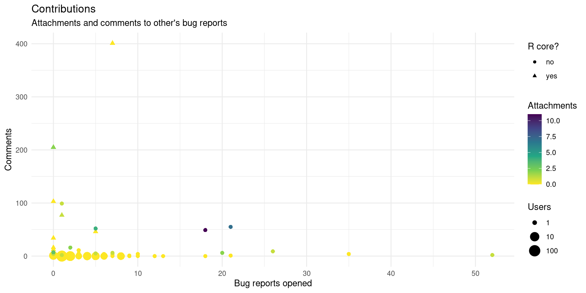

We can see that the R core members contribute a lot with many comments as previously explored. There is also a group of people consistently opening many bugs, and some users not in the R core contributing with many attachments.

If we check with the list above we can see these contributors activity:

p +     
    geom_text_repel(aes(open, comment, label = real_name), 
                    data = active_users_merged) +
    scale_y_log10()

Note that this plot is on log10 scale on the y axis.

I also received the question about how often bug submitters stay engaged after receiving a comment (or a patch).

user_engaged <- history |> 
    group_by(bug_id) |> 
    arrange(time) |> 
    summarize(opener = user[action == "open"],
        other_comments = any(opener != user & action == "comment"),
        r_core = any(r_core %in% user[user != opener]),
        # engaged = sum(user == opener & action != "open") > 1,
        when_o = min(which(!user[-c(1:2)] %in% opener)), # Skiping opening and first comment
        when_u = min(which(user[-c(1:2)] %in% opener)),
        when_u = ifelse(is.infinite(when_u), 0, when_u),
        when_s = min(which(action %in% c("ASSIGNED", "CLOSED"))-2),
        when_s = ifelse(is.infinite(when_s), 0, when_s),
        engaged = when_o < when_u,
        handled = when_s == when_o + 1
        ) |> 
    filter(other_comments) |> 
    ungroup()
user_engaged |> 
    count(engaged, name = "bugs") |> 
    mutate(engaged = ifelse(engaged, "yes", "no")) |> 
    knitr::kable()

engaged	bugs
no	409
yes	122

It seems that on most the bugs opened the submitter does not engage when they receive some feedback. This could be because the bug is fixed, bug 17393, or closed directly without fixing it, bug 17265, or because the user doesn’t reply to questions or feedback if asked ( 16441 ).

If we look at if after a new comment outside the original poster it is closed we can see better what happens

user_engaged |> 
    filter(!engaged) |> 
    count(handled, name = "bugs") |> 
    mutate(handled = ifelse(handled, "yes", "no")) |> 
    knitr::kable()

handled	bugs
no	177
yes	232

Most bug reports where users are not engaged (do not reply to comments) is due to it being handled (closed or assigned) on the first comment they receive.

We can make a table with the number of users that open the same number of bugs, some of which where handled (closed or assigned by those who can) and the percentage of said bugs that the original submitter stayed engaged on the bugs after someone else commented on their bugs. With this table we can see if there is more engagement when the bug reports are not closed or assigned on the first comment.

ue |> 
    count(handled_p, engaged_p, bugs, name = "users") |> 
    ggplot() + 
    geom_point(aes(handled_p, engaged_p, size = users, col = bugs)) +
    scale_x_continuous(labels = scales::label_percent(), limits = c(0, 1), 
                       expand = expansion(add = 0.05)) +
    scale_y_continuous(labels = scales::label_percent(), limits = c(0, 1), 
                       expand = expansion(add = 0.05)) +
    scale_size(trans = "log10") +
    scale_color_continuous(trans = "log10") +
    labs(x = "Handled", y = "Engagement", 
         title = "Engagement of users on their bugs", 
         subtitle = "And handling the bugs on the first comment.",
         size = "Users", col = "Bugs")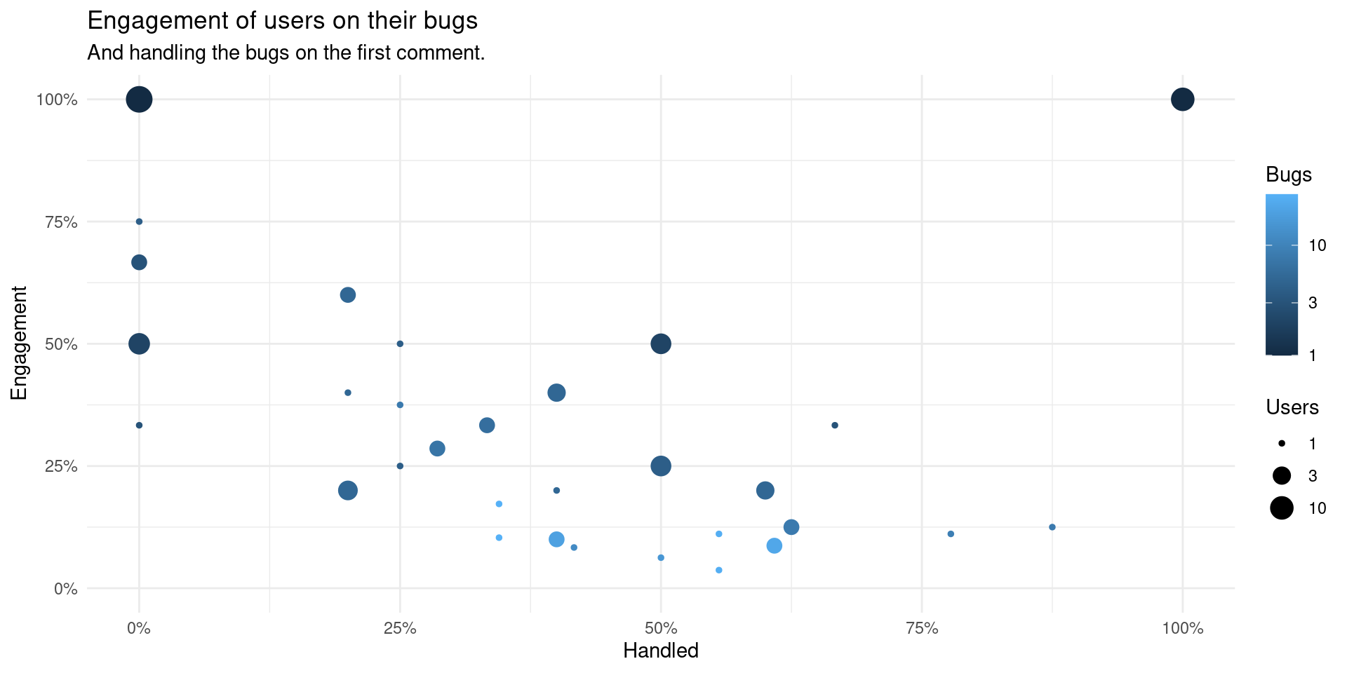

On the above plot it shows the users who engaged on bug reports and if their bugs where handled. Having more bugs handled seems to reduce users’ engagement. Probably users become more proficient submitting bugs reports (and/or patches) or could be also some effect of being more newer issues without time to engage.

Closing bug reports

As seen closing issues might have some effect on users. Issues might get closed for a variety of reasons as we have seen, but maybe there is some hint to something bugRzilla could help:

closing_time <- db_activity_bugs |> 
  group_by(bug_id) |> 
  summarize(
    creation_t = unique(creation_ts),
    closed_t = max(bug_when[added == "CLOSED"])) |> 
  ungroup() |> 
  mutate(diff_t = difftime(closed_t, creation_t, units = "hours")) |> 
  mutate(diff_t = if_else(closed_t < as.difftime(0, units = "hours") | is.na(closed_t), as.difftime("NA", units = "hours"), diff_t)) |> 
  mutate(closed = !is.na(diff_t == 0))

ggplot(closing_time) +
  geom_point(aes(x = creation_t, y = bug_id), col = "green", shape = 17, size = 1) +
  geom_point(aes(x = closed_t, y = bug_id), col = "red", size = 1, data = function(x){ filter(x, closed)}, alpha = 0.25) +
  scale_x_datetime(date_breaks = "1 year", date_labels = "%Y") +
  labs(x = element_blank(), y = "Bug", title = "Opening and closing bugs")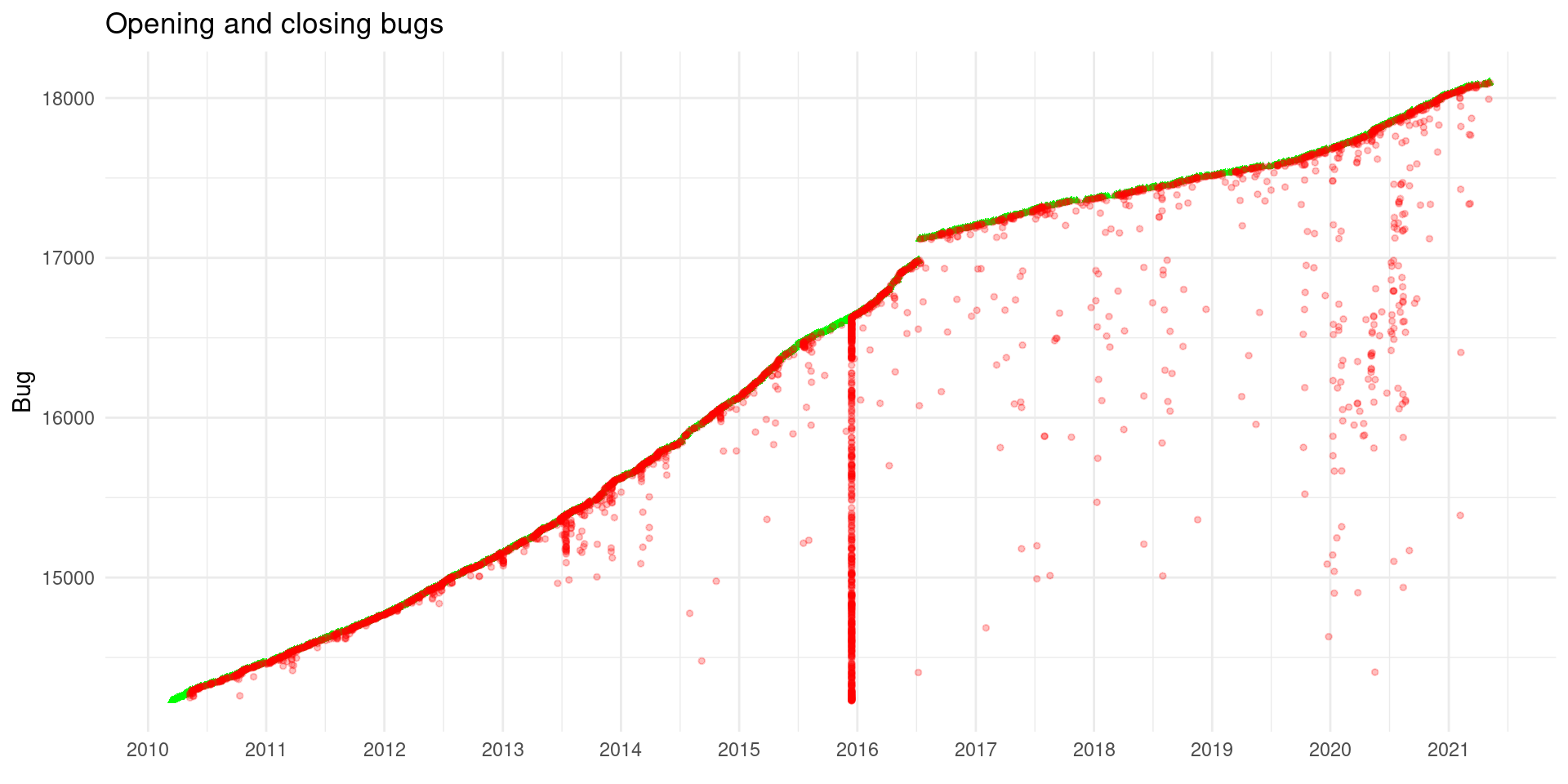

We can observe the rise of bug reports and the closing efforts. On mid 2014 there was some effort to close issues, and a big effort to close old issues on 2015-2016. More recently the effect of “R Can Use Your Help: Reviewing Bug Reports” is also appreciable but the closing effort seems more organic as it spans almost all 2020 closing old bug reports and it is not focused on a short span of time.

closing_time |>   
  filter(closed) |> 
  group_by(month = format(closed_t, "%Y-%m")) |> 
  count() |> 
  ggplot() +
  geom_col(aes(x = month, y = n)) +
  theme(axis.text.x = element_text(angle = 45, hjust = 1)) +
  scale_y_continuous(expand = expansion()) +
  labs(x = element_blank(), y = "Closed issues")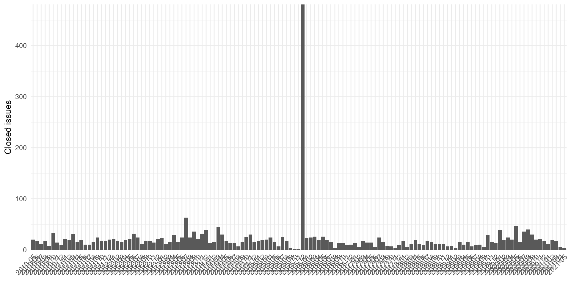

The big spike of near 500 closed issues on 2015-12 (presumably automatic), distorts a bit the graphic.

closing_time |>   
  filter(closed) |> 
  group_by(month = format(closed_t, "%Y-%m")) |> 
  count() |> 
  ggplot() +
  geom_col(aes(x = month, y = n)) +
  theme(axis.text.x = element_text(angle = 45, hjust = 1, vjust = 1)) +
  coord_cartesian(ylim = c(0, 65)) +
  scale_y_continuous(expand = expansion()) +
  labs(x = element_blank(), y = "Closed issues")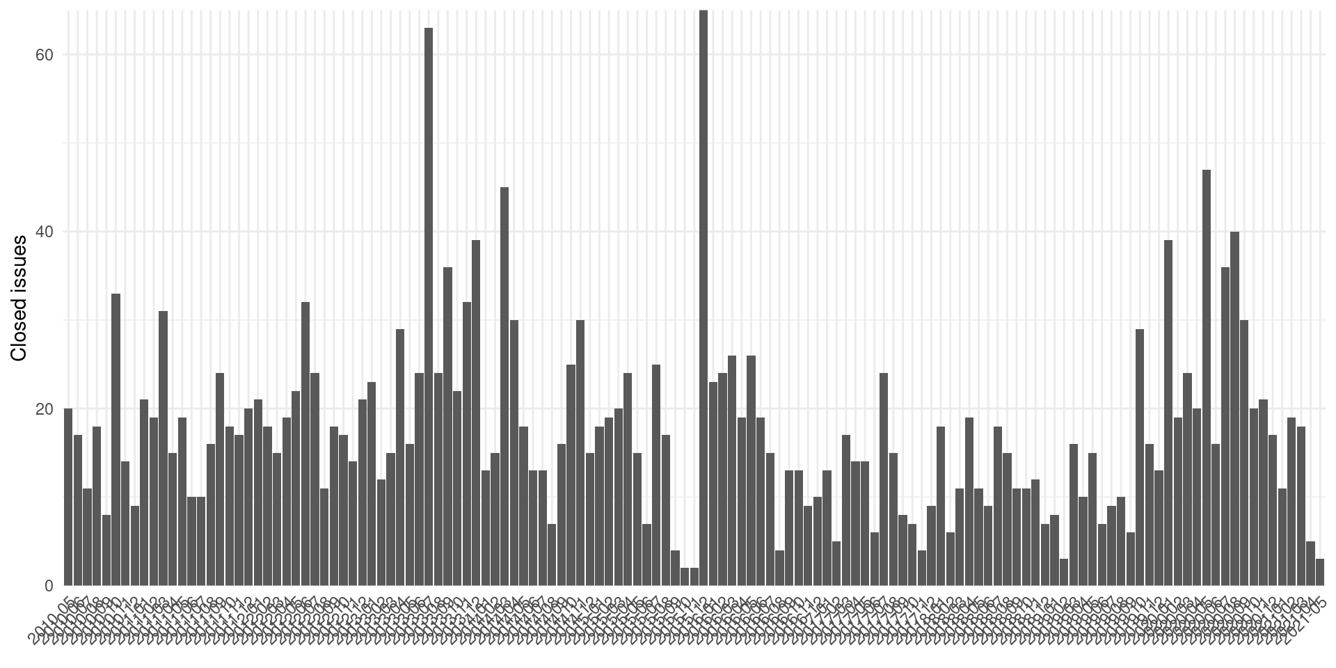

With near to 20 bugs closed each month, the question is which ones are closed faster? Perhaps some kind of resolution or status of bugs are closed sooner?

db_bugs4 |> 
  merge(closing_time, by = "bug_id", all.x = TRUE, all.y = FALSE) |> 
  filter(closed) |> 
  group_by(resolution, bug_severity) |> 
  summarize(f = as.numeric(median(diff_t))) |> 
  ungroup() |> 
  ggplot() +
  geom_tile(aes(bug_severity, resolution, fill = f)) +
  scale_fill_viridis_c(trans = "log10") +
  labs(x = "Severity", y = "Resolution", fill = "h", 
       title = "Median time till closing the issue")
## `summarise()` has grouped output by 'resolution'. You can override using the `.groups` argument.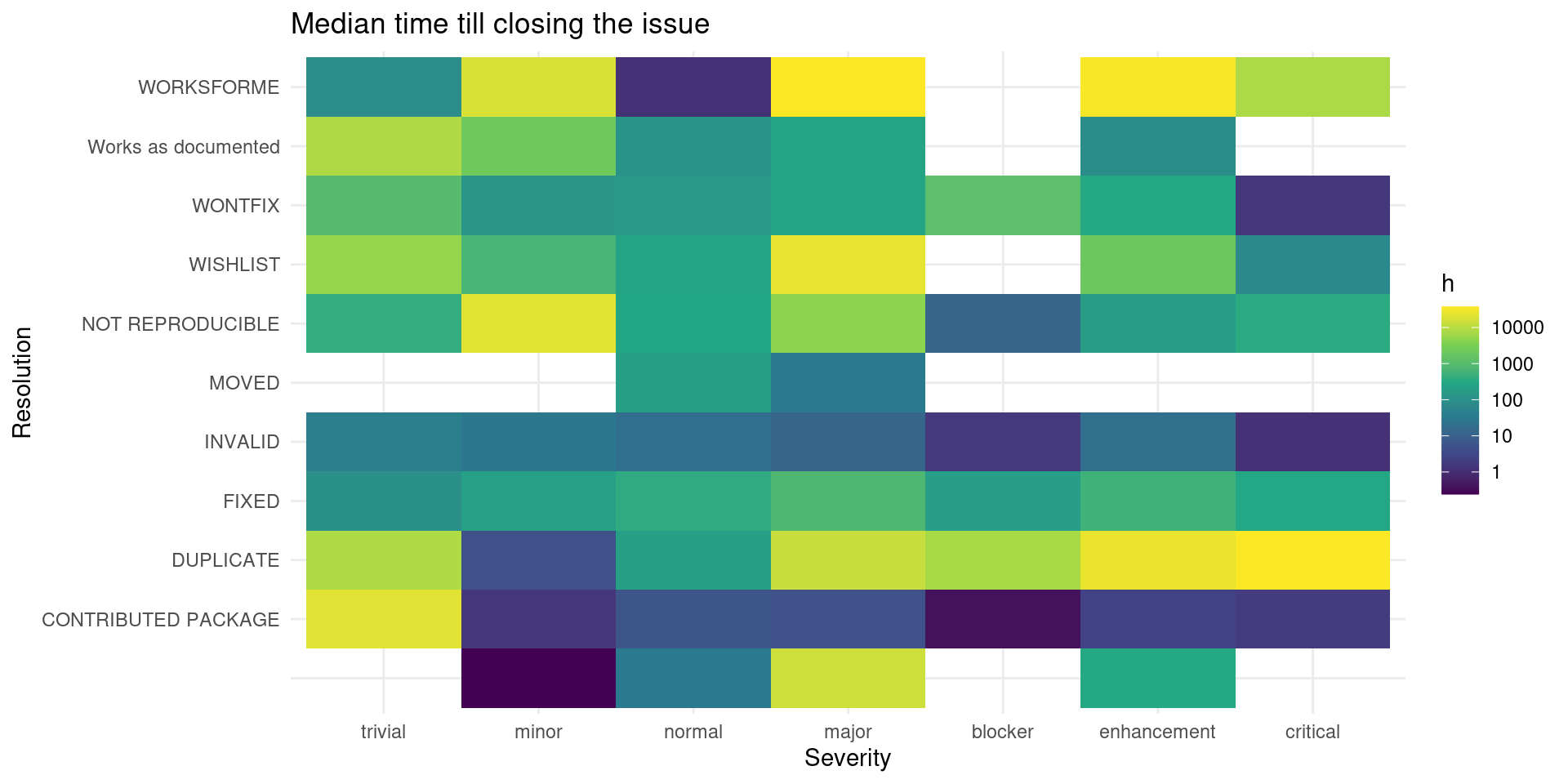

Usually it takes some time to close a bug report as duplicate. Maybe this is because one needs some familiarity with the previous reported bugs.

db_bugs4 |> 
  merge(closing_time, by = "bug_id", all.x = TRUE, all.y = FALSE) |> 
  filter(closed) |> 
  mutate(component_id = component_names[as.character(component_id)]) |> 
  group_by(op_sys, component_id) |> 
  summarize(f = as.numeric(median(diff_t)),
            cv = mean(diff_t)/sd(diff_t),
            n = n(),
            min = min(diff_t),
            max = max(diff_t)) |> 
  ungroup() |> 
  filter(n > 5) |> 
  ggplot() +
  geom_tile(aes(forcats::fct_reorder2(op_sys, cv, -n), 
                forcats::fct_reorder2(component_id, cv, -n),
                fill = f)) +
  scale_fill_viridis_c(trans = "log10") +
  labs(y = "Component", x = "OS", fill = "h", 
       title = "Median time till closing the issue", 
       subtitle = "For components and OS with more than 5 bugs reports") +
  theme(axis.text.x = element_text(angle = 45, hjust = 1))
## `summarise()` has grouped output by 'op_sys'. You can override using the `.groups` argument.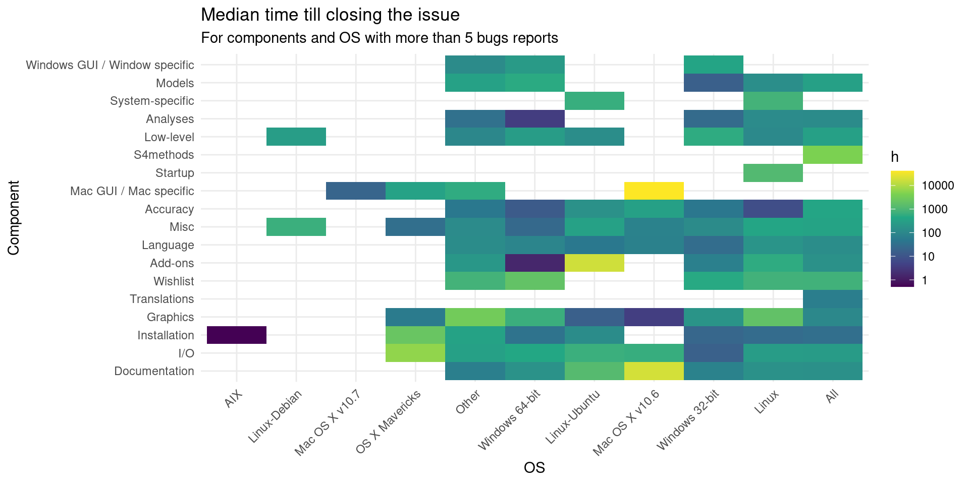

It was suggested that by looking by component and OS a pattern might emerge, but it doesn’t seem so. To visualize a little bit better the dispersion on each category we can plot them as boxplots:

comp_os <- db_bugs4 |> 
  merge(closing_time, by = "bug_id", all.x = TRUE, all.y = FALSE) |> 
  filter(closed) |> 
  mutate(component_id = component_names[as.character(component_id)],
         names = paste(component_id, op_sys, sep = "-"))
comp_os |> 
    count(op_sys, component_id, sort = TRUE) |> 
    filter(n > 5) |> 
    mutate(names = paste(component_id, op_sys, sep = "-"))
##            op_sys                  component_id   n
## 1             All                          Misc 135
## 2             All                     Low-level 132
## 3             All                 Documentation 124
## 4           Linux                     Low-level  90
## 5  Windows 64-bit Windows GUI / Window specific  87
## 6             All                      Wishlist  86
## 7             All                      Language  78
## 8           Linux                          Misc  76
## 9           Other                          Misc  56
## 10          Linux                  Installation  55
## 11          Linux                           I/O  46
## 12 Windows 64-bit                      Accuracy  46
## 13            All                      Graphics  45
## 14          Linux                      Graphics  42
## 15          Linux                 Documentation  40
## 16          Other                     Low-level  39
## 17            All                      Accuracy  38
## 18 Windows 64-bit                      Language  37
## 19 Windows 64-bit                          Misc  37
## 20          Linux                      Accuracy  36
## 21          Other                 Documentation  35
## 22 Windows 64-bit                           I/O  35
## 23 Windows 32-bit Windows GUI / Window specific  34
## 24          Linux                      Language  32
## 25 Windows 32-bit                      Graphics  32
##                                           names
## 1                                      Misc-All
## 2                                 Low-level-All
## 3                             Documentation-All
## 4                               Low-level-Linux
## 5  Windows GUI / Window specific-Windows 64-bit
## 6                                  Wishlist-All
## 7                                  Language-All
## 8                                    Misc-Linux
## 9                                    Misc-Other
## 10                           Installation-Linux
## 11                                    I/O-Linux
## 12                      Accuracy-Windows 64-bit
## 13                                 Graphics-All
## 14                               Graphics-Linux
## 15                          Documentation-Linux
## 16                              Low-level-Other
## 17                                 Accuracy-All
## 18                      Language-Windows 64-bit
## 19                          Misc-Windows 64-bit
## 20                               Accuracy-Linux
## 21                          Documentation-Other
## 22                           I/O-Windows 64-bit
## 23 Windows GUI / Window specific-Windows 32-bit
## 24                               Language-Linux
## 25                      Graphics-Windows 32-bit
##  [ reached 'max' / getOption("max.print") -- omitted 69 rows ]
comp_os |> 
    ggplot() +
    geom_boxplot(aes(x = as.numeric(diff_t), y = names, col = names))+
    # theme(axis.text.x = element_text(angle = 45, hjust = 1)) +
    scale_x_log10() +
    geom_vline(xintercept = 0) +
    guides(col = "none") +
    labs(x = "Hours", x = element_blank(), title = "Time to closing by OS and component") +
    scale_y_discrete(guide = guide_axis(n.dodge = 2))
## Warning: Transformation introduced infinite values in continuous x-axis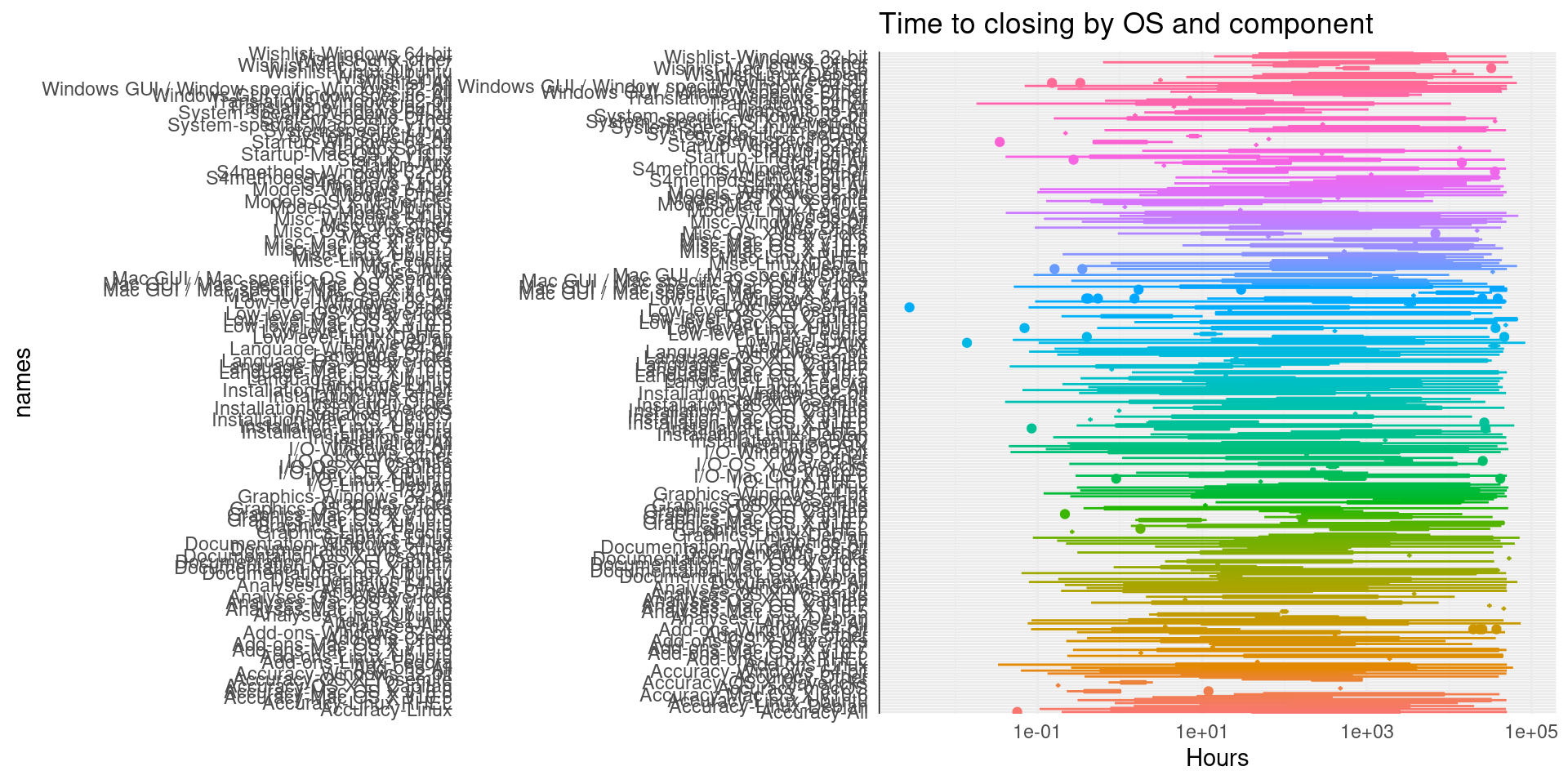

Not clear if there is a pattern there.

Looking at open bugs we can see this pattern of time:

db_bugs4 |> 
  merge(closing_time, by = "bug_id", all.x = TRUE, all.y = FALSE) |> 
  filter(!closed) |> 
  mutate(ct = difftime(as.Date("2021/03/25"), creation_t, units = "hours")) |> 
  group_by(resolution, bug_severity) |> 
  summarize(f = as.numeric(median(ct)), n = n()) |> 
  ungroup() |> 
  filter(n > 5) |> 
  ggplot() +
  geom_tile(aes(bug_severity, resolution, fill = f)) +
  scale_fill_viridis_c(trans = "log10") +
  labs(x = "Severity", y = "Resolution", fill = "h", 
       title = "Median time of open bug report")
## `summarise()` has grouped output by 'resolution'. You can override using the `.groups` argument.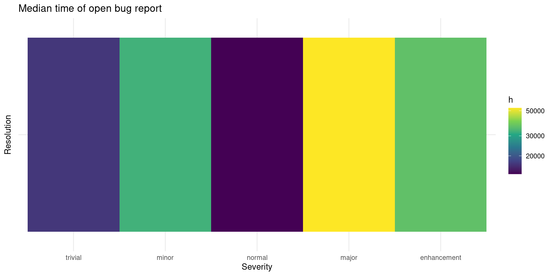

Bugs without resolution described as major are more time open, presumably because they take more time to fix too. Next are enhancements, which makes sense that enhancements take some time till they are incorporated to R source code. Perhaps is the effect of the recent call to help on Bugzilla but the normal bug reports seem to be the ones less time open.

speed <- db_bugs4 |> 
    arrange(bug_id) |> 
    mutate(n = 1:n(),
           days = difftime(creation_ts, min(creation_ts), units = "days"))
ggplot(speed) +
    geom_abline(intercept = 0, slope = 1, col = "red", linetype = 2) +
    geom_smooth(aes(days, n), method = "lm", formula = y ~ 0 + x) +
    geom_line(aes(days, n), size = 2) +
    labs(x = "Days", y = "Bugs", title = "Submission rate")
## Don't know how to automatically pick scale for object of type difftime. Defaulting to continuous.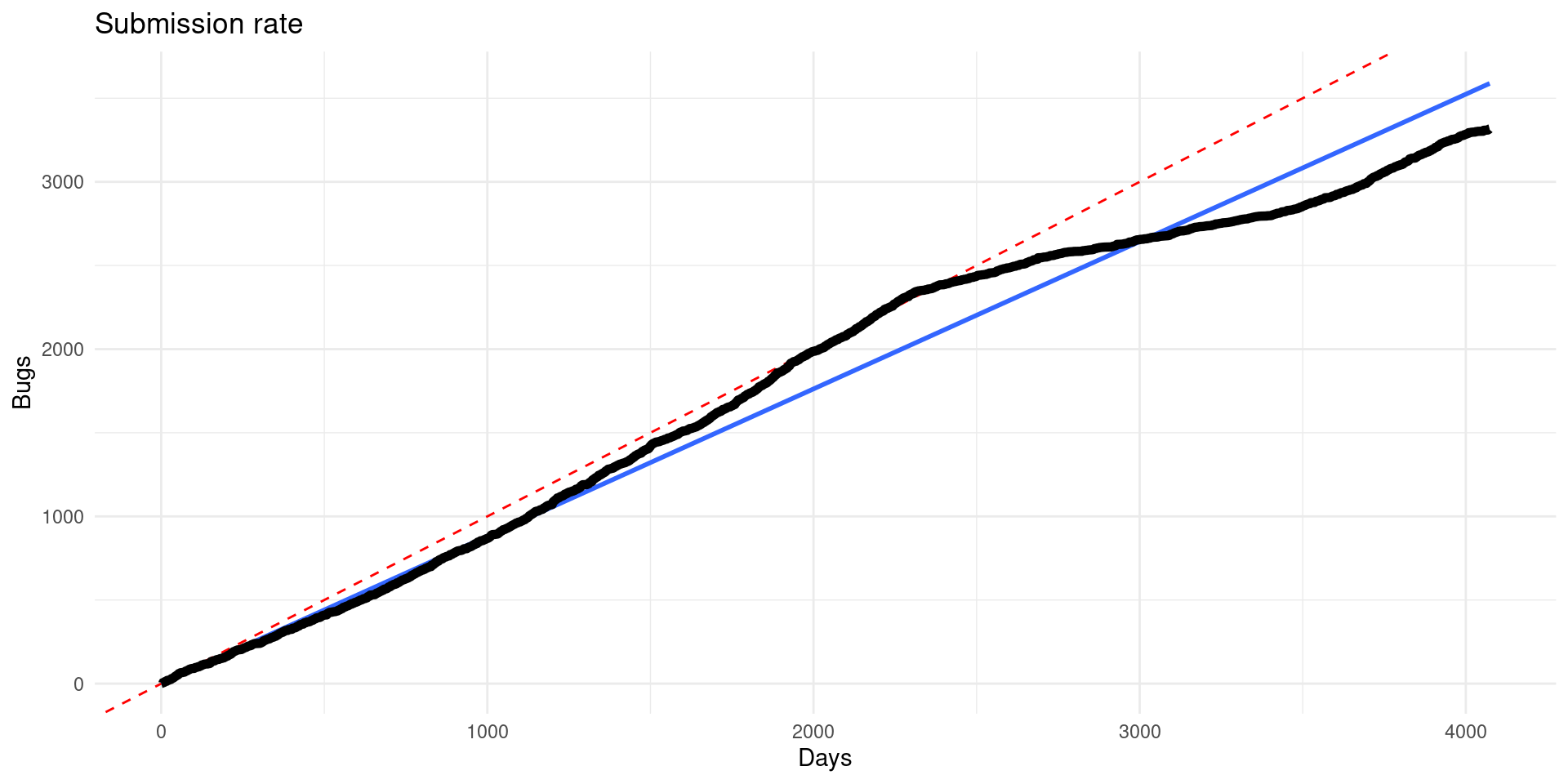

It seems that bugs were open close to one a day (red dashed line), there was a slow down between 2014 and 2020, but it seems that the peace has now recovered and raised again. Overall there is around 0.881 bugs reported per day since 2010 (blue continuous line).

Conclusion

There is room for improvements on the bug reporting process from users:

Include some efforts to trace the origin of the bug report.
Include a patch whenever possible or some suggestions how you think the bug could be fixed.
Give details of the kind of the bug or at least not always using the default options of the tracker.

Also some advice to bug reporters:

Don’t expect a fast comment if the issue is complicated.

If you explore the code, the warning tells us that there are some bugs without date of creation.↩︎
Note that this is only based on Bugzilla, and activity on Jitterbug might have been different.↩︎

Exploring the R Bugzilla

Lluís Revilla Sancho

8/28/2021 - 2022-01-12