1 Introduction
The goal of inteRmodel is to provide the tools required to search for models in the generalized canonical correlations as provided by the RGCCA package.
You can read more about canonical correlation at (Tenenhaus and Tenenhaus 2011).
In this use case we want to find the best model to relate the gene expression on a glioma with some repetitions at the DNA level, taking into account that these tumors are at three different locations. Our idea is that the location might influence the tumor.
2 Data format
We use the data used on the vignette of the RGCCA package. We need the samples in the rows and the variables in the columns:
data("ge_cgh_locIGR")
A <- ge_cgh_locIGR$multiblocks
Loc <- factor(ge_cgh_locIGR$y)
levels(Loc) <- colnames(ge_cgh_locIGR$multiblocks$y)
A[[3]] = A[[3]][, -3]
names(A)[3] <- "Loc"
With these steps we read and prepare the data for the sgcca and rgcca function.
3 Workflow
The workflow is as follows:
- Selecting the interaction-model
- Evaluation of the models
- Tuning the weight in the different interaction models
- Comparison of the different models after bootstrapping
These steps are explained in detail in the next sections.
3.1 Null hypothesis
Then we need to encode our hypothesis in a model, which takes the shape of a matrix. To ease the design of this model there are several functions available. The most important one is subSymm, which makes substitutions on symmetric matrices.
C <- matrix(0, nrow = 3, ncol = 3, dimnames = list(names(A), names(A)))
model0 <- subSymm(C, "GE", "CGH", 1)
model0 <- subSymm(model0, "GE", "Loc", 1)
model0
#>     GE CGH Loc
#> GE   0   1   1
#> CGH  1   0   0
#> Loc  1   0   0
Here we hypothesize that the Agriculture and the industry are linked and that the agriculture is linked with the political block.
3.2 Search models
Now we look for the model that best relates these data.
out_model <- search_model(A = A, c1 = c(.071, .2, 1), scheme = "horst",
               scale = FALSE, verbose = FALSE,
               ncomp = rep(1, length(A)),
               bias = TRUE)
This quickly explores over the 20 different models that could be the best ones. We can see that our hypothesis is in the upper middle:
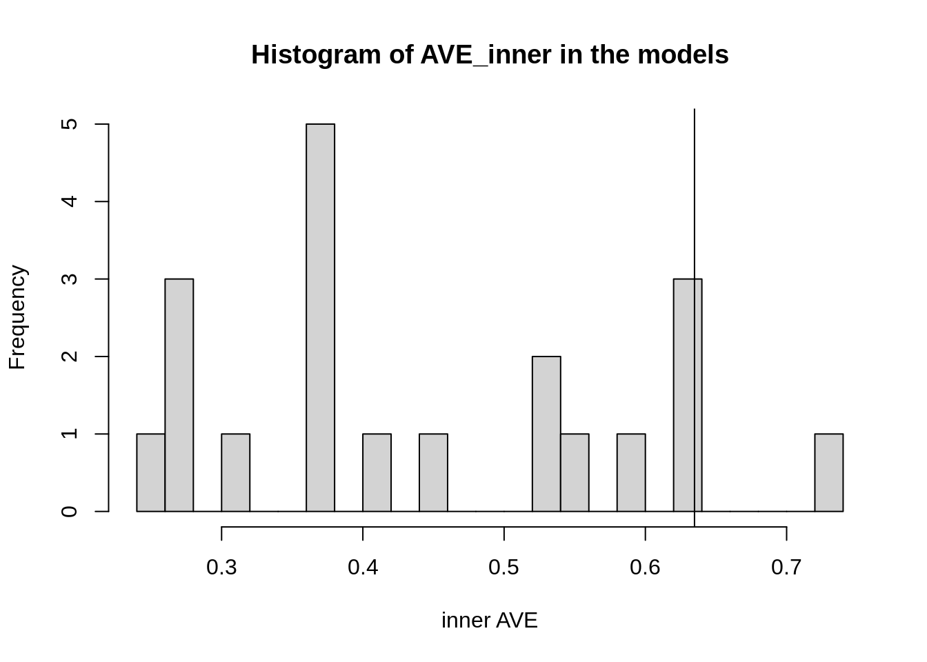
Figure 1: Histogram of the different inner AVE values of each model.
According to this, a better model would then be:
columns <- grep("var", colnames(out_model))
model <- symm(C, out_model[which.max(out_model$AVE_inner), columns])
model
#>     GE CGH Loc
#> GE   0 0.0 1.0
#> CGH  0 0.0 0.5
#> Loc  1 0.5 0.0
A model that instead of the expected relation between Agriculture and Industry block, they are both related to the Political block.
3.3 Refinement of the model
We further explore the relationships in this model:
out_best <- iterate_model(C = model, A = A, c1 = c(.071,.2, 1),
                          scheme = "horst",
                          scale = FALSE, verbose = FALSE,
                          ncomp = rep(1, length(A)),
                          bias = TRUE)
We can see that usually the model is around 0.4 inner AVE.
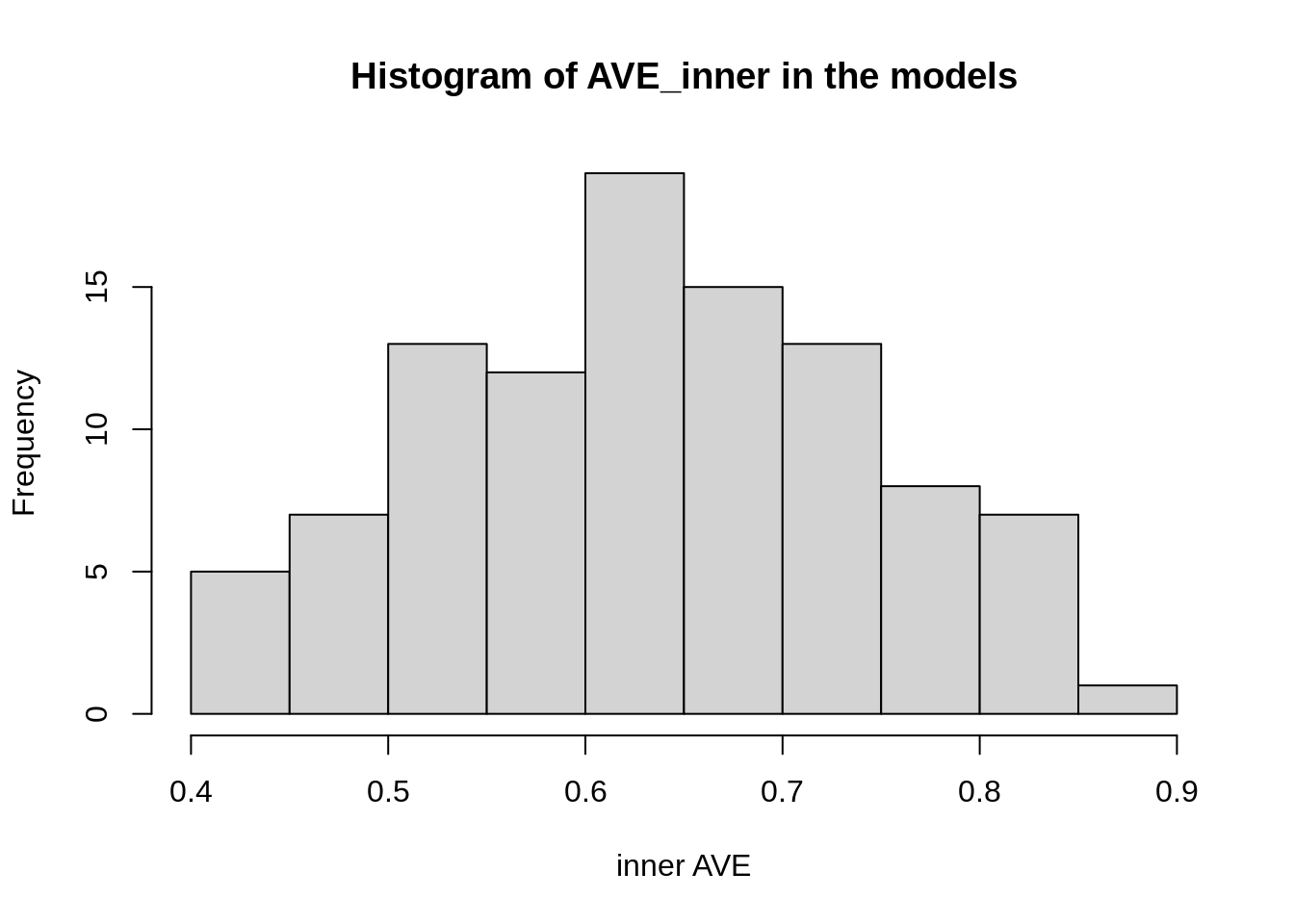
Figure 2: Histogram of the different inner AVE values of the same model but with different weights for those connections.
The best model would then be:
3.4 Evaluate stability
A next step would be to see if some models are better than the others, something along these lines but with more iterations.
index <- boot_index(nrow(A[[1]]), 10)
bs0 <- boot_index_sgcca(index, A = A, C = model0, c1 = c(.071,.2, 1))
bs1 <- boot_index_sgcca(index, A = A, C = model, c1 = c(.071,.2, 1))
bs2 <- boot_index_sgcca(index, A = A, C = model2, c1 = c(.071,.2, 1))
3.4.1 Stability
We can see that they have different distributions:
plot(c(0.6, 0.9), c(0.05, 0.15), type = "n", xlab = "inner AVE", ylab = "outer AVE",
     main = "Bootstrap of models")
points(bs0$AVE, pch = 16, col = "red")
points(bs1$AVE, pch = 16, col = "green")
points(bs2$AVE, pch = 16)
legend("topright", legend = c("model2", "model", "model0"),
       fill = c("black", "green", "red"))

df <- rbind(
  cbind.data.frame(bs0$AVE, Model = "model 0"),
  cbind.data.frame(bs1$AVE, Model = "model 1"),
  cbind.data.frame(bs2$AVE, Model = "model 2"))
agg <- aggregate(df[, 1:2], list(Model = df$Model), mean)
points(agg[, 2:3], pch = 17, col = c("red", "green", "black"), cex = 1.5)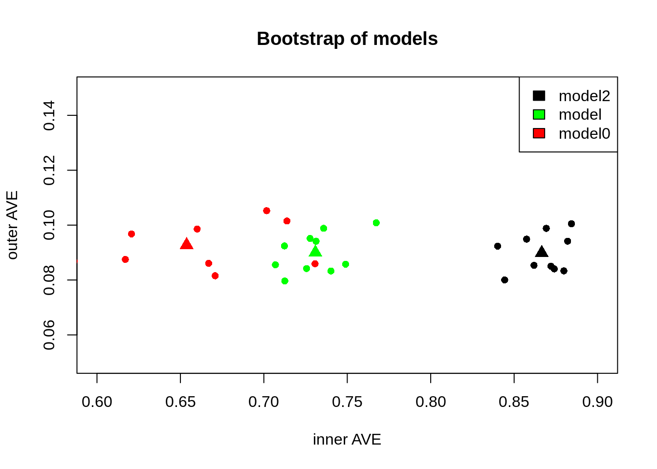
Figure 3: Comparison of the models, our null hypothesis along the model with higest inner AVE. Triangles show the centroid of each group
This suggests that the model2 has a higher inner AVE than the model0. With more iterations we could see if there is a tendency of a model to be more centered than the others. So, indicating that the model can better find the relationship between the blocks regardless of the input data.
3.4.2 Features
We can now analyze the canonical correlation for the weight of each variable.
m2 <- RGCCA::sgcca(A, model2, c1 = c(.071,.2, 1), scheme = "horst",
               scale = TRUE, verbose = FALSE, ncomp = rep(1, length(A)),
               bias = TRUE)
m0 <- RGCCA::sgcca(A, model0, c1 = c(.071,.2, 1), scheme = "horst",
               scale = TRUE, verbose = FALSE, ncomp = rep(1, length(A)),
               bias = TRUE)
We can now explore the position of each sample:
pars <- par(mfrow = c(1, 2))
plot(m0$Y[[1]][, 1], m0$Y[[2]][, 1], type = "n", xlab = "Block1 Comp1",
     ylab = "Block2 Comp1", main = "Initial model")
abline(h = 0, v = 0)
text(m0$Y[[1]][, 1], m0$Y[[2]][, 1], labels = Loc, col = as.numeric(Loc) + 1)

plot(m2$Y[[1]][, 1], m2$Y[[2]][, 1], type = "n", xlab = "Block1 Comp1",
     ylab = "Block2 Comp1", main = "Final model")
abline(h = 0, v = 0)
text(m2$Y[[1]][, 1], m2$Y[[2]][, 1], labels = Loc, col = as.numeric(Loc) + 1)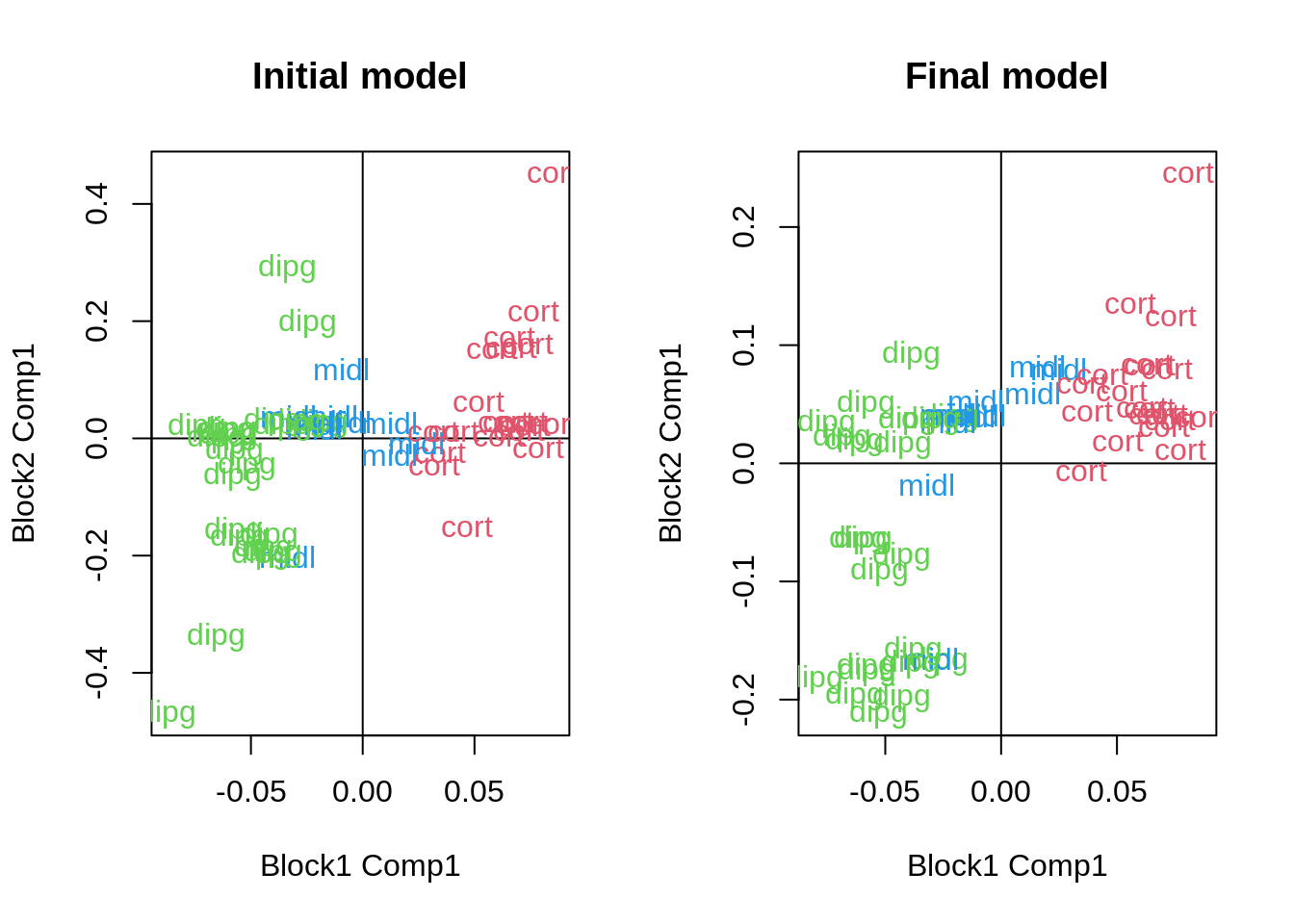
Figure 4: Differences on the canonical dimensions of the samples
Although there is a relative difference in the general outcome, what has changed more is the importance of each variable. As we can see here:
par(pars)
plot(m0$a$CGH[, 1], m2$a$CGH[, 1], main = "CGH variables importance",
     xlab = "model0", ylab = "model2", pch = 16)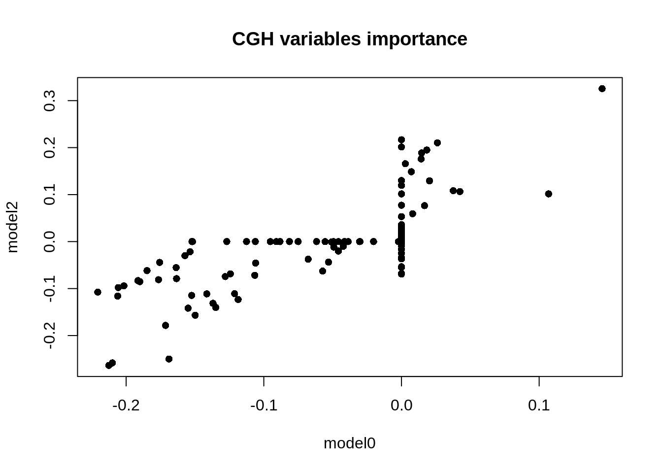
Figure 5: Comparison of the weights of the CGH variables
Where some variables that had a weight of 0 in model 0 become important and some variables that were important that no longer have any weight on the model 2.
4 Conclusion
Finding a different model that explains your data better challenges the assumptions about the data. By comparing models, we can learn which blocks of variables are connected thus showing new relationships. These new relationships consider the same variables but with different importance, which, with the right model, should be more accurate.
5 Session Info
sessionInfo()
#> R version 4.1.3 (2022-03-10)
#> Platform: x86_64-pc-linux-gnu (64-bit)
#> Running under: Ubuntu 20.04.4 LTS
#>
#> Matrix products: default
#> BLAS:   /usr/lib/x86_64-linux-gnu/blas/libblas.so.3.9.0
#> LAPACK: /usr/lib/x86_64-linux-gnu/lapack/liblapack.so.3.9.0
#>
#> locale:
#>  [1] LC_CTYPE=C.UTF-8       LC_NUMERIC=C           LC_TIME=C.UTF-8
#>  [4] LC_COLLATE=C.UTF-8     LC_MONETARY=C.UTF-8    LC_MESSAGES=C.UTF-8
#>  [7] LC_PAPER=C.UTF-8       LC_NAME=C              LC_ADDRESS=C
#> [10] LC_TELEPHONE=C         LC_MEASUREMENT=C.UTF-8 LC_IDENTIFICATION=C
#>
#> attached base packages:
#> [1] stats     graphics  grDevices utils     datasets  methods   base
#>
#> other attached packages:
#> [1] inteRmodel_0.1.1.9002
#>
#> loaded via a namespace (and not attached):
#>  [1] knitr_1.37          magrittr_2.0.2      MASS_7.3-55
#>  [4] BiocParallel_1.28.3 lattice_0.20-45     R6_2.5.1
#>  [7] rlang_1.0.2         fastmap_1.1.0       stringr_1.4.0
#> [10] highr_0.9           tools_4.1.3         parallel_4.1.3
#> [13] grid_4.1.3          xfun_0.30           RGCCA_2.1.2
#> [16] cli_3.2.0           jquerylib_0.1.4     htmltools_0.5.2
#> [19] yaml_2.3.5          digest_0.6.29       Matrix_1.4-0
#> [22] sass_0.4.0          evaluate_0.15       rmarkdown_2.13
#> [25] stringi_1.7.6       compiler_4.1.3      bslib_0.3.1
#> [28] jsonlite_1.8.0